A Data Visualization Approach for Intersection Analysis using AIS Data

Ricardo Cardoso Pereira, Pedro Henriques Abreu, Evgheni Polisciuc and Penousal Machado

Centre for Informatics and Systems of the University of Coimbra, Department of Informatics Engineering,

olo II - Pinhal de Marrocos, 3030-290 Coimbra, Portugal

Keywords:

Automatic Identiﬁcation System, Data Visualization, Data Processing, Magniﬁed Fish-Eye Lens.

Abstract:

Automatic Identiﬁcation System data has been used in several studies with different directions like trafﬁc

forecasting, pollution control or anomalous behavior detection in vessels trajectories. Considering this last

subject, the intersection between vessels is often related with abnormal behaviors, but this topic has not been

exploited yet. In this paper an approach to assist the domain experts in the task of analyzing these intersections

is introduced, based on data processing and visualization. The work was experimented with a proprietary

dataset that covers the Portuguese maritime zone, containing an average of 6460 intersections by day. The

results show that several intersections were only noticeable with the visualization strategies here proposed.

1 INTRODUCTION

The Automatic Identiﬁcation System (AIS) is an in-

ternational standard for communication between ves-

sels and terrestrial stations developed to improve mar-

itime safety (Tetreault, 2005). AIS data contains all

the necessary information for mapping the trajecto-

ries followed by each vessel and the general maritime

trafﬁc of any sea, and for that reason it has been used

in several studies. The majority of these studies are

focused particularly in trafﬁc analysis and forecasting

(Sang et al., 2016), pollution control (Busler et al.,

2015), fusion of different maritime data sources (Xu

et al., 2015) or identiﬁcation of vessels’ anomalous

behaviors (Handayani et al., 2013; Soleimani et al.,

2015). Regarding this last topic, there are a set of

common abnormal activities involving two vessels

that were identiﬁed by the domain experts (e.g. navy

operators), such as two vessels sailing very close to

each other, which could be an indicator that an illegal

trade is happening, and two vessels crossing trajec-

tories, especially if one of them goes from the coast

to the intersection zone and comes back after a short

period of time, which could be an indicator that this

vessel went to the zone to pick up some illegal goods

left by the other one. These activities are often related

to abnormal intersections between them. Published

works in the data visualization ﬁeld have only been

focused in new representations of the trafﬁc situation

from speciﬁc areas of interest (Willems et al., 2009;

Gao and Shiotani, 2013; Chen et al., 2016), with mi-

nor or no emphasis on any type of anomalous behav-

iors, including intersections. This work proposes a

new approach, based on data processing and visual-

ization, to assist the detection of anomalous behaviors

by domain experts, with a particular interest on inter-

sections. This approach solves the following prob-

lems from the visualization perspective:

• To process the raw AIS data and extract the inter-

sections from it, a set of data processing tasks are

introduced;

• To detect and unveil the intersections within the

visual clutter created by all the trajectories, a vi-

sual search strategy based on a magniﬁed ﬁsh-eye

lens is proposed;

• To properly analyze individual intersections by

displaying the direction and the speed of the ves-

sels, an animated strategy is introduced that dis-

plays the trajectories of the vessels over time;

• To decide which areas of the sea have a higher

probability of containing anomalous intersec-

tions, a visual selection strategy based on high

density areas associated with an abnormality level

is introduced.

The approach was experimented with a propri-

etary dataset that contains data from the Portuguese

maritime zone, collected between February 22 and

March 12 of 2012. An average of 6460 intersections

per day were detected, and the majority are only vis-

ible with the proposed visualization strategies. Two

case studies are presented as a proof of concept.

The remainder of the paper is organized in the fol-

208

Pereira, R., Abreu, P., Polisciuc, E. and Machado, P.

A Data Visualization Approach for Intersection Analysis using AIS Data.

DOI: 10.5220/0007312802080215

In Proceedings of the 14th International Joint Conference on Computer Vision, Imaging and Computer Graphics Theory and Applications (VISIGRAPP 2019), pages 208-215

ISBN: 978-989-758-354-4

lowing way: Section 2 presents recent related works

that exploit AIS data with visual strategies, Section

3 introduces the proposed approach for the intersec-

tions analysis, Section 4 presents a proof of concept

with real data and describes the dataset, and Section 5

presents the conclusions and future directions.

2 RELATED WORK

Regarding AIS data visualization, most works are fo-

cused on visual strategies to display the trafﬁc pat-

terns, where the trend is to explore density-based vi-

sualizations. Chen et al. (Chen et al., 2016) intro-

duced the concept of summary visualization where

relevant patterns are visualized through density heat

maps that highlight the high-speed and slow-down ar-

eas. Willems et al. (Willems et al., 2009) proposed

a new kernel density method based on the speed of

the vessels that is able to measure the contribution of

each vessel in each point of the map. Jiacai et al. (Ji-

acai et al., 2012) introduced a new data visualization

model that divides the region of interest into a grid

and calculates an index of the maritime trafﬁc situ-

ation for each cell. Gao and Shiotani (Gao and Sh-

iotani, 2013) introduced the usage of 3D visualiza-

tions to analyze speciﬁc vessels and provide a trust-

ful representation of their environment. Fiorini et al.

(Fiorini et al., 2016) proposed a pipeline of actions to

go from raw AIS data to a proper visualization of the

vessels routes, using only open-source tools, being the

ﬁnal result an interactive web-like geographical visu-

alization. Riveiro and Falkman (Riveiro and Falkman,

2009) introduced an interactive visual analytics model

that is able to present the density probability of each

combination of several AIS kinematic values.

As stated before, the works described are only fo-

cused on presenting the trafﬁc situation of speciﬁc ar-

eas of interest, through different visual strategies that

are often density-based and interactive. In general,

minor or no emphasis is given to anomalous behav-

iors, being this a direction yet to be explored. The ap-

proach proposed on this work exploits AIS intersec-

tions as anomalies, which consists of a novelty point.

3 PROPOSED APPROACH

The proposed approach for intersections analysis is

composed by the extraction tasks and three distinct

visualization strategies to address the problems de-

scribed in section 1. This section describes with detail

each of these components.

In order to display the AIS positions several deci-

sions must be made regarding the usage of the visual

variables. These decisions are common to the three

strategies proposed in this work, and are based on

the visual semiology concepts proposed by Jacques

Bertin (Bertin, 1983). AIS positions are represented

by the cartesian coordinate system, which means that

a map projection needs to be applied to the origi-

nal geographic coordinates (latitude and longitude) of

each AIS position. In this work the Spherical Merca-

tor projection is used, mainly because the more im-

portant interactive maps platforms, like Google Maps

and OpenStreetMaps, also use it. Regarding the vi-

sual marks used to represent the AIS positions and in-

tersections, it was decided to represent each position

through a circle with a radius of one pixel and each in-

tersection with the same shape but with a radius of ﬁve

pixels. The intersections are displayed in solid black

and each type of vessel has a different color used to

paint its positions, meaning that this visual variable is

being used for association purposes.

3.1 Intersections Extraction

Before applying any visual method, the AIS raw data

must be processed in order to extract the intersections.

A ﬁrst necessary task is to remove the duplicated posi-

tions of each vessel. This is an important step because

repeated AIS positions will lead to the detection of

multiple intersections that are actually the same. This

work proposes an approach that isolates the positions

of each vessel and detects the ones that are within a

minimum time and distance gaps, being these ones la-

beled as repeated. The time gap is calculated by the

absolute difference between the time-stamps of both

positions, which are in the UNIX Epoch time format.

To calculate the distance between these positions the

Haversine formula is used since it considers the cur-

vature of Earth. This algorithm requires as parameters

the minimum time and distance gaps. The used values

are 15 seconds and one meter and they were obtained

empirically. The second and most important task is to

detect and extract each intersection between different

vessels. For this purpose a new algorithm was intro-

duced that detects an intersection when two positions

of different vessels have time and distance gaps below

the minimum thresholds passed as parameters. Both

gaps are calculated using the same methods from the

previous task that removes the duplicated positions.

The used values for these parameters are 30 minutes

and one kilometer respectively, and they were also ob-

tained empirically. This algorithm does not take into

account the direction of the intersection, considering

A to B and B to A as different, when they are actually

A Data Visualization Approach for Intersection Analysis using AIS Data

209

the same. The algorithm could deal with this issue

but that would have impact on its performance and,

for that reason, the issue is ﬁxed in a third task that it-

erates over the intersections, transforms them into sets

and calculates a hash for each one. Duplicated hashes

are then removed.

3.2 Unveil the Intersections

With all the AIS positions displayed in the same

screen a lot of visual clutter may exist. As a conse-

quence, it can become difﬁcult to detect the intersec-

tions and even more difﬁcult to analyze each one in-

dividually. Therefore, a ﬁrst necessary step is to cre-

ate the means for the users to efﬁciently search and

focus on speciﬁc intersections. In this work the ﬁsh-

eye lens (Bettonvil, 2005; Altera, 2008) is used for

this purpose. This type of lens applies a convex ef-

fect to the image, creating the illusion that it has the

shape of a sphere, an effect commonly called barrel

distortion. With this effect the center of the image be-

comes the focus, while the boundaries become grad-

ually distorted. Consequently, the center of the image

becomes more zoomed, with the cost of losing some

resolution. When combining this type of lens with the

movement of the mouse, the users can focus on spe-

ciﬁc AIS positions and intersections, surpassing the

visual clutter issue. Different distortions with spe-

ciﬁc characteristics can be applied with a ﬁsh-eye lens

through different mapping functions. The most pop-

ular ones are the equidistant, equisolid, orthographic

and stereographic (Bettonvil, 2005). The used func-

tion in this approach is the orthographic mapping and

it was chosen empirically. The conclusion was that

this mapping is the one that better distorts the bound-

aries of the image through a more exaggerated cur-

vature, which gives more focus and zoom to the cen-

ter. To apply the ﬁsh-eye effect two parameters are

required: the focal length f

and the width radius of

the lens r

. Both parameters are correlated and their

values can be obtained empirically. Figure 1 shows

an example of the ﬁsh-eye lens applied with different

conﬁgurations. On the left an image is displayed with

the ﬁsh-eye effect using f

= 4 and r

= 5, and on the

right the same projection is used but with f

= 2. In

this last case, with an increased focal length the zoom

was much higher and the pixel interpolation method -

which is part of the ﬁsh-eye projection - was unable to

ﬁll in all the missing gaps, creating the “black pixels”

visible on the image. In this work the ﬁsh-eye param-

eters used are f

= 3 and r

= 5, and the effect is only

applied to a speciﬁc area of interest, which is the area

of the map that the user wants to analyze. This area is

deﬁned by the mouse position (mouse

, mouse

) and

Figure 1: On the left an image displayed with the ﬁsh-eye

effect applied using f

= 4 and r

= 5, and on the right the

same projection but with f

= 2.

by a radius mouse

that will create a circle around it.

An example of this behavior is presented on Figure

2, with the original area displayed on the left and the

same area with the ﬁsh-eye effect on the right.

Figure 2: On the left the original area in analysis. On the

right the same area with the ﬁsh-eye effect applied and the

intersections identiﬁed.

The application of the ﬁsh-eye lens gives the user

a way to focus and zoom on a speciﬁc area, but the

level of magniﬁcation may not be enough for an ef-

ﬁcient analysis. Increasing the zoom only by deﬁn-

ing an higher focal length has growth limitations and

will lead to the problem presented on the right im-

age of Figure 1. Therefore, this work combines the

ﬁsh-eye effect with levels of magniﬁcation. The key

concept is to render the area of the map in analy-

sis n times, where each time the level of zoom is

increased by a scalar zoom

. The zoom of the ge-

ographical positions is handled by the majority of

the map projections available (including the Spheri-

cal Mercator) through a scalar that indicates the mag-

niﬁcation to be applied. The maximum number of

levels can be predeﬁned or it can be adjusted while

the zoom increases, with this last strategy having a

performance cost. Assuming that zoom

is the initial

zoom of the area that corresponds to the level n = 0,

the zoom of each n level is calculated using the for-

mula zoom

= zoom

+ (n ∗ zoom

). An important as-

pect of this method is that the magniﬁcation effect

needs to be applied to the center of the area in anal-

ysis, otherwise it would start to change. To ensure

this aspect the cartesian coordinates of each position

in each level need to be shifted according to a point

of reference from the base level (n = 0). This point

of reference (x

, y

) is the AIS position that has the

IVAPP 2019 - 10th International Conference on Information Visualization Theory and Applications

210

minimum euclidean distance between the ﬁxed mouse

position (mouse

, mouse

) and itself. Considering a

point (x

, y

) on any given level and the point of ref-

erence (x

, y

) on the same level, the shift formulas

are x

new

= (x

− x

+ (x

− mouse

) + mouse

) and

new

= (y

− y

+ (y

− mouse

) + mouse

). These

equations also have an adjustment between the point

of reference in the base level and the mouse position

because this point may not be exactly in the center of

the area. To navigate between the levels of magniﬁca-

tion the user will ﬁrst ﬁx the area in analysis through

a mouse click and, after that, two controls to change

the zoom will appear. Each time the zoom level is up-

dated the ﬁsh-eye effect is reapplied. This behavior

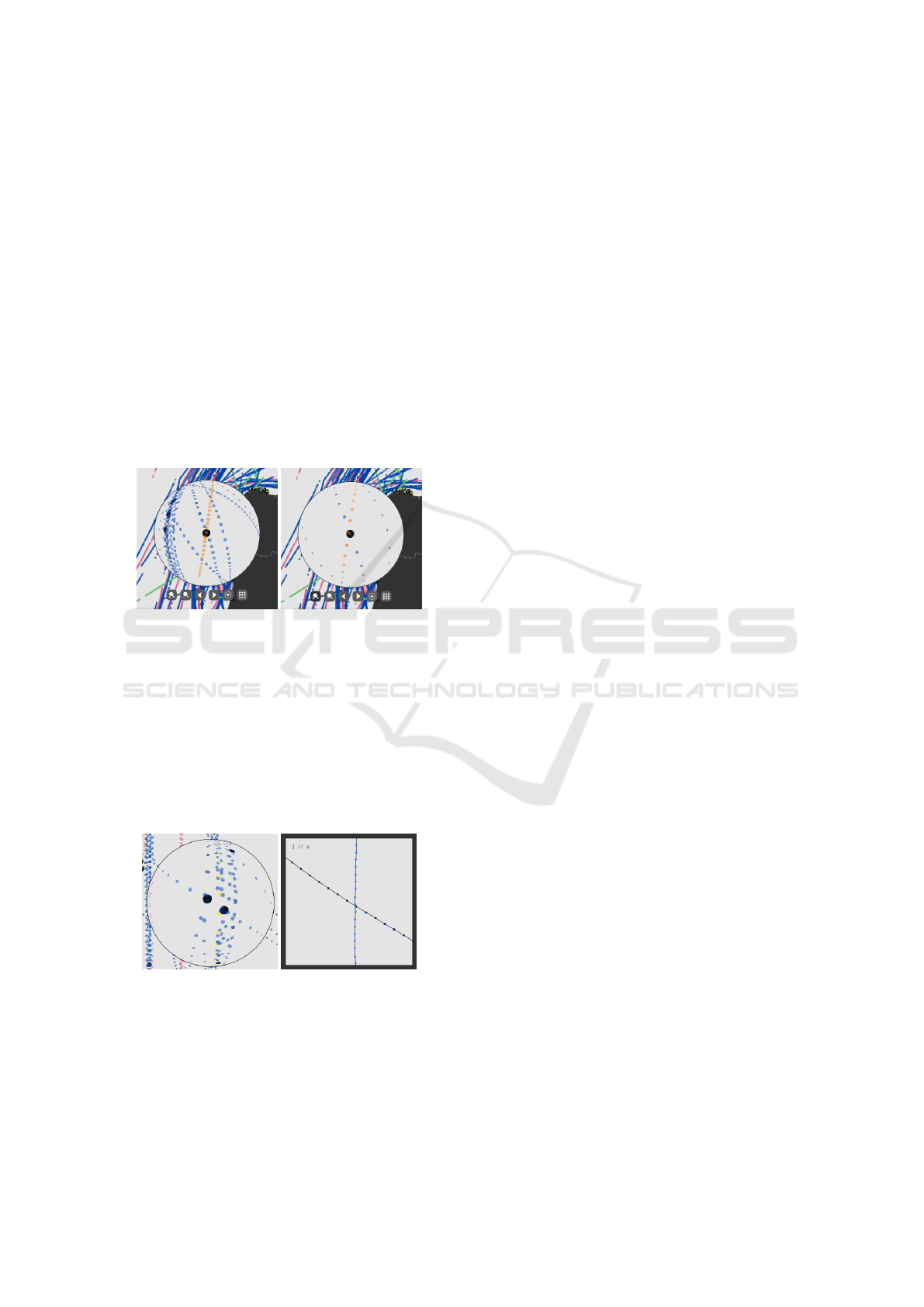
is presented on Figure 3, displaying the desired effect

on the left with the default magniﬁcation and the same

effect on the right with the third level of zoom. When

Figure 3: On the left the ﬁsh-eye effect with the default

magniﬁcation. On the right the same effect but with the

third level of zoom.

the area in analysis is ﬁxed the intersections inside it

are presented individually on a detail lens located on

the top-right corner of the screen. This lens has the

same level of zoom used on the ﬁsh-eye lens and al-

lows the user to analyze each intersection individually

without the visual clutter, as Figure 4 shows. The user

can change intersections using two controls displayed

next to the zoom ones (see Figure 3). When the trajec-

Figure 4: On the left are all the intersections visible through

the ﬁsh-eye lens. On the right a speciﬁc intersection is iso-

lated through the detail lens.

tories displayed on the detail lens are from two ves-

sels of the same type, the collision of colors can make

the identiﬁcation of the positions from each vessel a

difﬁcult task. To ﬁx this issue a lighter and darker

color were created for each type of vessel based on

the original palette. These colors are then used when

the above scenario happens.

3.3 Individual Intersections Analysis

Visualizing the vessels trajectories of an intersection

with a static approach has several limitations regard-

ing the amount of features that can be displayed. With

the existing visual variables only the positions of the

vessel and its type can be presented. This means that

two very important features for behavior analysis are

ignored: the speed and the direction. To present these

two features this work uses the motion variable, com-

bined with the position and the orientation, through

an animation approach that allows the visualization

of the vessels moving over time. For the animation

to be performed the period in analysis is divided into

15 minutes frames. This interval was used because

it includes more than one position by vessel (often

two to four positions), which allows a better under-

standing of the trajectories evolution in terms of di-

rection. Each frame contains the vessels positions

from its time interval and the ones from the previous

frames, and it is displayed a quarter of a second after

the previous one, creating the desired motion effect.

Each vessel position is drawn through a circle with a

radius of seven pixels. The positions from the cur-

rent time interval are drawn with an opacity of 100%

but the ones that are from previous frames are drawn

black with an opacity of only 10% (this value was ob-

tained empirically). This creates a trace effect that

allows the perception of how the vessels are moving

over time without losing track of their position in the

current frame.

The vessels new positions and directions are auto-

matically displayed through the animation as a con-

sequence of the motion effect. The points added in

each frame are enough to understand the direction

of a vessel because these new points will change the

orientation of the trajectory. However, the speed at-

tribute requires further efforts to be visible. An ap-

proach was developed where the speed is represented

by the accumulative opacity of the vessels trace over

time. Assuming that a vessel reports its positions in

a ﬁxed period of time (for instance, each ﬁve min-

utes), if this vessel is moving slowly the reported po-

sitions will be very close to each other. However, if

the vessel is moving fast these positions will be far

from each other. When all the positions are drawn at

the same time on the trace of the vessel, the ones that

are overlaid will generate a higher opacity because

their individual colors are blended. This means that

the areas of the trajectories where the transparency of

the trace is lower are the ones where the vessels are

A Data Visualization Approach for Intersection Analysis using AIS Data

211

moving slower, because more points were overlaid for

this effect to happen. On the contrary, a trace with

a higher transparency corresponds to a vessel mov-

ing faster. As stated before, this speed visualization

approach only works if the time-span between each

position of a vessel is ﬁxed, which is a problem be-

cause the AIS communication periods are not consis-

tent. To ﬁx this issue a cubic spline interpolation is

applied to every trajectory to generate the missing po-

sitions. As stated in the literature (Zhang et al., 2017;

Sang et al., 2012), this type of interpolation is the

one that adjusts better to the reconstruction of AIS

trajectories, offering just some limitations in the pres-

ence of very tight curves. This interpolation creates a

piecewise function, which means that it deﬁnes sev-

eral small sub-intervals through the domain of x, and

has an individual polynomial of degree three for each

one. This aspect is important to make the ﬁnal func-

tion more smooth and better suitable for curves. The

interpolation is made individually for the latitude and

the longitude, being these variables the output y of the

generated functions and the timestamp in seconds the

input x. The polynomial coefﬁcients of both functions

are calculated with all the AIS positions of the respec-

tive vessel. Each of these positions is then compared

with the one immediately after and, if the time gap

between them is over ﬁve minutes, new positions are

generated through the interpolated functions, with in-

tervals of also ﬁve minutes until the gap is ﬁlled. This

ﬁve minutes period was deﬁned empirically. Figure 5

shows an example of a frame from an animation with

four vessels sailing at different speeds. It is visible

that the tanker vessel (the pink one) in the middle is

sailing at a low speed, maintaining a route in a very

small area, while the other two tankers sailed faster.

The cargo vessel (the dark blue one) started slow but

increased the speed roughly in the middle of the tra-

jectory.

Figure 5: An example of a frame from an animation with

vessels sailing at different speeds.

3.4 Areas with Anomalous Intersections

The visual search mechanism already described is im-

portant to identify and isolate intersections for indi-

vidual analysis, but when a big quantity of intersec-

tions exist within the visible data it may be difﬁcult

to decide where to start the search. With this issue

in mind, an approach to identify areas with a higher

probability of having anomalous intersections is pro-

posed in this work. The approach can be described in

the following steps:

1. Identify the areas, for each day, where the quantity

of intersections is higher;

2. Analyze if those areas are constant over the days;

3. Deﬁne more frequent areas as less probable of

having abnormal behaviors;

4. Visualize the areas and the abnormality levels.

Regarding the ﬁrst step, areas with a higher quan-

tity of intersections can be seen as clusters with a

higher density. Therefore, a density-based cluster-

ing strategy was used to extract these areas from the

data. Density Based Spatial Clustering of Applica-

tions with Noise (DBSCAN) has been used exten-

sively with AIS data and had shown good results (Pal-

lotta et al., 2013; Gonzalez et al., 2014), which made

it the most obvious choice for the algorithm to be

used. However, this algorithm requires the minimum

number of points by clusters (MinPts) and the dis-

tance between each point and its neighbors (ε), and

this last one is not easy to estimate because there are

zones of the map where the distance between the ves-

sels positions is supposed to be lower (e.g. near the

ports) and zones where it is supposed to be higher

(e.g. high sea corridors). For this reason the Hier-

archical Density Based Spatial Clustering of Applica-

tions with Noise (HDBSCAN) was also considered,

because it uses an approach where the ε value is not

required as a parameter and the clusters can have dif-

ferent densities. Both algorithms were experimented

with different conﬁgurations of the parameters to al-

low a more effective choice of clusters. Regarding

the values of MinPts, it was observed by visual anal-

ysis that, with the exception of ports, there were no

considerable areas with more than 100 intersections.

Therefore, this value was used as a maximum and the

MinPts was experimented with four values: 25, 50,

75 and 100. Regarding the values of ε for the DB-

SCAN, a maximum of 750 meters was deﬁned and the

parameter was experimented with three values: 250,

500 and 750 meters. Notice that the algorithms were

applied individually for the AIS data of each day. To

choose the better algorithm and conﬁguration the sil-

houette coefﬁcient was applied to the retrieved clus-

ters, using an euclidean distance for the calculations.

The average coefﬁcient results and standard devia-

tions are presented on Table 1 for the best four con-

ﬁgurations of both algorithms. The results show that

the HDBSCAN with MinPts = 75 was the conﬁgu-

ration with an higher silhouette coefﬁcient average

IVAPP 2019 - 10th International Conference on Information Visualization Theory and Applications

212

while maintaining an acceptable standard deviation.

Therefore, it was chosen for the clusters extraction.

Table 1: Silhouette results for HDBSCAN and DBSCAN.

Algorithm MinPts ε Avg. Std.

HDBSCAN 75 NA 0.525 0.084

HDBSCAN 100 NA 0.507 0.081

DBSCAN 25 750 0.499 0.070

DBSCAN 75 750 0.473 0.077

Regarding the second step, the key idea was to as-

sociate a frequency to each cluster of each day. To

calculate this frequency (F

) the formula on Equation

1 was proposed.

Number of days where the cluster exists

Total number of days

(1)

Considering the necessary parameters for the formula

above, the total number of days with AIS data is a

known value but the number of days where each clus-

ter exists needs to be calculated. For this purpose a

new algorithm was developed that receives a cluster

from a day, the clusters of the remaining days and an

overlap threshold (between zero and one). The key

idea is to evaluate if the given cluster exists on other

days by calculating the area of intersection between it

and each of the remaining clusters. This area is then

converted to a percentage by dividing it with the area

of the given cluster, and if this percentage is greater

than the overlap threshold it is considered that the

cluster exists on the selected day. The overlap thresh-

old is important in this analysis because it is highly

unlikely that two clusters have the exact same shape,

which would be necessary for a degree of 100% of

overlap. Moreover, the goal is to identify if an area

that has an high density in one day also has it in other

days, and for that reason a total overlap is not required

since the same area may be within a bigger or smaller

cluster on others days. For these reasons, the value

of this threshold was deﬁned as 50%. Notice that

this algorithm could use the overlap of each individ-

ual point from the clusters for the calculations, but

the required time for the algorithm to compute would

be unfeasible. Therefore, the area from the clusters

was considered to calculate the overlap, but this is not

an immediate operation. In this approach the area is

obtained from the convex hulls of the clusters points,

which are extracted using the Graham’s Scan algo-

rithm (Graham, 1972). The shape of the convex hull

adapts well to the clusters, because it considers all the

boundaries and is able to represent them without re-

strictions (being an irregular polygon, it can assume

any convex shape). Considering that the coordinates

from the vertices are known, the formula presented on

Equation 2 can be used to calculate the area. Notice

that the coordinates must be applied in counterclock-

wise order around the polygon, using the ﬁrst point

also as the last one.

n−1

∑

k=0



∗ y

k+1

− y

∗ x

k+1



(2)

With the frequency of each cluster calculated, the

third step was addressed by associating less common

clusters as more likely to include abnormal behaviors.

This concept has been used in other studies and re-

lies on the fact that an area where an higher density

of intersections is often found should be considered

less probable of being abnormal when compared to

one where this higher density happens as an excep-

tion. Therefore, the level of abnormality of each clus-

ter was calculated based on the frequency using the

formula on Equation 3.

= 1 − F

(3)

Finally, addressing the fourth step, to visualize

these clusters the convex hulls are drawn on the plat-

form and the visual variable color was used for the

representation of the abnormality levels. These levels

were discretized into four intervals, namely [0, 0.25[,

[0.25, 0.50[, [0.50, 0.75[ and [0.75, 1]. A gradient of

the color red was created with four levels, each one

for a speciﬁc interval, where the ﬁrst level (light red)

is the lowest and the fourth level (dark red) is the high-

est. The convex hull drawn for each cluster is ﬁlled

with the color that matches its interval of abnormal-

ity. Figure 6 shows an example with two areas drawn

on the platform. The one from the left has a lower

level of abnormality compared to the one on the right.

Figure 6: An example with two abnormal areas drawn on

the platform.

4 PROOF OF CONCEPT

The proposed approach was implemented in Java with

Processing 3 and tested with real data. An usage

example of the implementation is presented in the

following video: https://vimeo.com/304586547.

The used proprietary dataset has AIS data from the

Portuguese maritime zone collected between Febru-

ary 22 and March 12 of 2012. It contains positions for

A Data Visualization Approach for Intersection Analysis using AIS Data

213

the nine types of vessels available but with very un-

balanced quantities for each type, being these the pre-

dominant three: cargos with 52%, tankers with 21%

and special crafts with 8%. Analyzing the trajecto-

ries of the vessels, the following statistics can also be

obtained: the dataset contains a total of 9394 trajec-

tories, the average duration of a trajectory is 1.5 days

and the average number of trajectories by day is 1085.

Considering the 20 days of data available, each

day has an average of 6460 intersections. Figure

7 displays several AIS trajectories from vessels that

sailed through the main corridor of the Portuguese

maritime area on February 22 of 2012. These mar-

itime corridors are speciﬁc areas of the sea where the

vessels are supposed to sail, and the trafﬁc density on

them is usually very high. The selected day has 4838

Figure 7: Visualization of several AIS trajectories.

intersections in a total of 86652 positions, which rep-

resents a ratio of 5.6%. Apparently the area marked

by the black square contains only cargo vessels (the

dark blue ones) and a ﬁshing vessel (the green one).

Moreover, it appears that the ﬁshing vessel may even-

tually intersect with several cargos. However, when

the intersections are activated and the ﬁsh-eye lens

is applied on the black square area with at least one

level of zoom, an unexpected intersection is revealed.

Figure 8 shows this intersection on the ﬁsh-eye lens

(left image) and on the detail lens (right image). The

Figure 8: Individual analysis of the intersection. On the

left the magniﬁed ﬁsh-eye lens is applied. On the right the

intersection is isolated through the detail lens.

intersection between the ﬁshing vessel and the pas-

sengers vessel (the yellow one) was hidden in the vi-

sual clutter created by the trajectories of the remain-

ing ones. Without the usage of the magniﬁed ﬁsh-eye

lens it would be very difﬁcult to detect and analyze

this intersection.

Fishing vessels can be particularly hard to analyze

considering that their trajectories are very irregular

when comparing, for example, with cargos or tankers.

Figure 9 (left image) displays AIS trajectories from

March 10 of 2012. Notice that the cargos and tankers

were removed from the screen. The area marked by

Figure 9: On the left the visualization of the AIS ﬁshing tra-

jectories. On the right the intersections and the high density

area of the same trajectories.

the black square on the Figure 9 appears to contain

a trajectory from a ﬁshing vessel. However, when

the intersections are displayed, the screen shows that

there are more than one trajectory from ﬁshing ves-

sels in that area and, more importantly, they intersect

in several points. Moreover, the area is considered

to have a high density of intersections and the red

color indicates that the level of abnormality is three

out of four. Figure 9 (right image) shows these inter-

sections and the high density area. When the ﬁsh-eye

lens is applied on the area the intersections are iso-

lated through the detail lens. Figure 10 shows all in-

tersections on the ﬁsh-eye lens (left image) and only

the ﬁrst intersection on the detail lens (right image).

Notice that, being the two vessels from the same type,

each one is painted with a light or dark green. The an-

Figure 10: Detection and isolation of the ﬁrst intersection.

On the left the magniﬁed ﬁsh-eye lens is applied. On the

right the ﬁrst intersection is isolated through the detail lens.

imation of trajectories was applied to the intersection

and, as Figure 11 shows, one of the vessels is always

following the other. This pattern could be an impor-

tant aspect to conﬁrm or discard the behavior as sus-

picious. The speed of the vessels is more or less con-

stant with the exception of some turning points where

it decreases.

IVAPP 2019 - 10th International Conference on Information Visualization Theory and Applications

214

Figure 11: Three frames of the animation from the isolated

intersection.

5 CONCLUSIONS

This paper proposes the ﬁrst approach that is focused

on analyzing intersections between vessels through

data processing and interactive visualization strate-

gies. The approach consists of several data processing

tasks that extract the intersections from the raw AIS

data, a visual search strategy based on a magniﬁed

ﬁsh-eye lens, an animation strategy that allows an in-

dividual analysis of the trajectories and a visual selec-

tion method based on high density areas and their ab-

normality levels. The experiments showed that these

new strategies help on the detection and analysis of

intersections that otherwise would be hidden in the

visual clutter. In the future an aspect to explore is

the evaluation of the usability and efﬁciency of the

proposed strategies with real users, particularly with

domain experts, in order to understand if they have

difﬁculties during the process. Another direction to

explore is to obtain more AIS datasets, which will al-

low new experiments in other contexts.

REFERENCES

Altera (2008). A ﬂexible architecture for ﬁsheye correction

in automotive rear-view cameras. Technical report,

Altera Corporation.

Bertin, J. (1983). Semiology of Graphics: Diagrams, Net-

works, Maps. University of Wisconsin Press.

Bettonvil, F. (2005). Fisheye lenses. WGN, Journal of the

International Meteor Organization, 33:9–14.

Busler, J., Wehn, H., and Woodhouse, L. (2015). Track-

ing vessels to illegal pollutant discharges using multi-

source vessel information. The International Archives

of Photogrammetry, Remote Sensing and Spatial In-

formation Sciences, 40(7):927.

Chen, C., Wu, Q., Zhou, Y., and Mao, Z. (2016). Informa-

tion visualization of ais data. In Logistics, Informatics

and Service Sciences (LISS), 2016 International Con-

ference on, pages 1–8.

Fiorini, M., Capata, A., and Bloisi, D. D. (2016). Ais

data visualization for maritime spatial planning (msp).

International Journal of e-Navigation and Maritime

Economy, 5:45–60.

Gao, X. and Shiotani, S. (2013). An effective presentation

of navigation information for prevention of maritime

disaster using ais and 3d-gis. In Oceans-San Diego,

2013, pages 1–6.

Gonzalez, J., Battistello, G., Schmiegelt, P., and Biermann,

J. (2014). Semi-automatic extraction of ship lanes and

movement corridors from ais data. In Geoscience and

Remote Sensing Symposium (IGARSS), 2014 IEEE In-

ternational, pages 1847–1850.

Graham, R. L. (1972). An efﬁcient algorith for determin-

ing the convex hull of a ﬁnite planar set. Information

processing letters, 1(4):132–133.

Handayani, D. O. D., Sediono, W., and Shah, A. (2013).

Anomaly detection in vessel tracking using support

vector machines (svms). In Advanced Computer Sci-

ence Applications and Technologies (ACSAT), 2013

International Conference on, pages 213–217.

Jiacai, P., Qingshan, J., Jinxing, H., and Zheping, S. (2012).

An ais data visualization model for assessing maritime

trafﬁc situation and its applications. Procedia Engi-

neering, 29:365–369.

Pallotta, G., Vespe, M., and Bryan, K. (2013). Vessel pat-

tern knowledge discovery from ais data: A framework

for anomaly detection and route prediction. Entropy,

15(6):2218–2245.

Riveiro, M. and Falkman, G. (2009). Interactive visualiza-

tion of normal behavioral models and expert rules for

maritime anomaly detection. In Computer Graphics,

Imaging and Visualization, 2009. CGIV’09. Sixth In-

ternational Conference on, pages 459–466.

Sang, L.-Z., Yan, X.-P., Mao, Z., and Ma, F. (2012). Restor-

ing method of vessel track based on ais information.

In Distributed Computing and Applications to Busi-

ness, Engineering & Science (DCABES), 2012 11th

International Symposium on, pages 336–340.

Sang, L.-z., Yan, X.-p., Wall, A., Wang, J., and Mao, Z.

(2016). Cpa calculation method based on ais position

prediction. The Journal of Navigation, 69(6):1409–

1426.

Soleimani, B. H., De Souza, E. N., Hilliard, C., and Matwin,

S. (2015). Anomaly detection in maritime data based

on geometrical analysis of trajectories. In Information

Fusion (Fusion), 2015 18th International Conference

on, pages 1100–1105.

Tetreault, B. J. (2005). Use of the automatic identiﬁcation

system (ais) for maritime domain awareness (mda).

In OCEANS, 2005. Proceedings of MTS/IEEE, pages

1590–1594.

Willems, N., Van De Wetering, H., and Van Wijk, J. J.

(2009). Visualization of vessel movements. In Com-

puter Graphics Forum, volume 28, pages 959–966.

Xu, W., Zhong, D., Wu, S., and Ni, H. (2015). A track

fusion method of a vessel. In Sixth International Con-

ference on Electronics and Information Engineering,

volume 9794, page 97941E.

Zhang, D., Li, J., Wu, Q., Liu, X., Chu, X., and He, W.

(2017). Enhance the ais data availability by screening

and interpolation. In Transportation Information and

Safety (ICTIS), 2017 4th International Conference on,

pages 981–986.

A Data Visualization Approach for Intersection Analysis using AIS Data

215

REFERENCES

Altera (2008). A flexible architecture for fisheye correction