Dynamic Path Planning with

Stable Growing Neural Gas

Carsten Hahn, Sebastian Feld, Manuel Zierl and Claudia Linnhoff-Popien

Mobile and Distributed Systems Group, LMU Munich, Munich, Germany

Keywords:

Path Planning, Autonomous Agents, Robots, Machine Learning, Collision Avoidance, Neural Networks.

Abstract:

This paper considers the problem of path planning under dynamic aspects. We propose ”Neural Gas Dynamic

Path Planning” (NGDPP), a novel algorithm that continuously provides a valid path between two points inside

an environment that transforms in an unpredictable manner. These transformations can occur due to both,

changes in the environment’s shape and moving collision objects. The algorithm incorporates several tech-

niques: Neural Gas, a dynamic discretization method; the A* Algorithm, a path planning algorithm for graphs;

and the Potential Field method, which facilitates the avoidance of collisions. We empirically evaluate the pro-

posed algorithm under various aspects providing performance information and guidance about situations and

applications beneﬁting from the algorithm. The evaluation reveals that NGDPP is a solid algorithm for path

planning in dynamic environments. Yet, the algorithm is based on heuristic information, i.e. a optimal result

in term of the path length cannot be guaranteed.

1 INTRODUCTION

Autonomous path planning is an important topic in

artiﬁcial intelligence research. From an evolutionary-

biological point of view there is the assumption that

the brain in living beings has arisen, among other

things, from the need to move (Legendre et al.,

1994). It is therefore logical that one goal in the ﬁeld

of Artiﬁcial Intelligence is to make purposeful and

meaningful movements automatically, i.e. computer-

controlled. A meaningful movement is only possible

if it has been planned beforehand, which leads to the

path planning problem.

We consider a problem domain consisting of an

autonomous agent that is able to move freely in a two

dimensional ﬂoor plan. The agent’s goal is to navigate

to given targets. Besides, an agent can either locate

itself inside the ﬂoor plan or knows at least its starting

position. We also allow that the walkable area can

change dynamically. These changes may occur due to

new areas that are made available or due to blockades

that separate the previously walkable area. The agent

shall adapt its plan to these changes. Finally, the agent

should neither collide with static obstacles nor with

dynamic obstacles like other agents.

In the following, the problem domain will be split

into three subproblems: a) Discretization of the con-

tinuous domain into a graph structure to ease compu-

tation , b) Path planning on the previously generated

graph structure, and c) Deployment of a suitable col-

lision avoidance strategy.

We propose a complete solution (namely NGDPP)

to the described problem domain that combines ex-

isting methods for the individual subtasks. We show

the beneﬁts arising by the combination of the chosen

methods. Furthermore we propose improvements for

the method chosen to discretize the continuous do-

main, namely Stable Growing Neural Gas (SGNG).

The paper is structured as follows. In Section II

common related approaches are outlined. Our ap-

proach as well as the used methods are presented in

Section III. This is followed by an evaluation in Sec-

tion IV. The paper is concluded in Section VI, where

also clues for future work are given.

2 RELATED WORK

There are multiple existing approaches that solely

treat one of the named subproblems. We focus on two

of the most common approaches for the discretization

and path planning in a continuous domain.

The Probabilistic Roadmap (PRM) (Kavraki et al.,

1996) method is a path planning algorithm for con-

tinuous spaces. The algorithm quantizes the space

by randomly setting nodes and connecting all exist-

138

Hahn, C., Feld, S., Zierl, M. and Linnhoff-Popien, C.

Dynamic Path Planning with Stable Growing Neural Gas.

DOI: 10.5220/0007313001380145

In Proceedings of the 11th International Conference on Agents and Artiﬁcial Intelligence (ICAART 2019), pages 138-145

ISBN: 978-989-758-350-6

ing nodes within a predeﬁned distance with an edge,

if the space allows it. Disjoint graphs, that possibly

occur, are connected in a posterior step. The pro-

cedure might produce many redundant edges which

densely cover certain areas of the space. Since the

graph created by the Probabilistic Roadmap is only

a snapshot of space in time, the question arises of

how to deal with dynamically changing spaces. In

this case, it is necessary to recalculate the roadmap

unless one has speciﬁc information about the nature

of the changes. Such a complete recalculation is very

inefﬁcient. However, there are procedures that make

the replanning of Probabilisic Roadmaps more efﬁ-

cient (Belghith et al., 2006). These are essentially

based on accelerating the path planning phase by us-

ing dynamic graph-based path planning algorithms

that do not require a complete recalculation of the

path (Likhachev et al., 2005).

Similar to the Probabilistic Roadmap, so-called

Rapidly Exploring Random Trees (RRT) (LaValle,

1998) are also based on the random generation of

waypoints. The intention behind RRT was to include

physical phenomena that inﬂuence real path planning

directly into the planned path. The path calculated

by a Probabilistic Roadmap may have sudden turns at

a certain angle: a path that a real agent (e.g. a car)

with properties such as speed, acceleration or braking

distance may not be able to drive. RRT is therefore

particularly suitable for non-holonomic systems. As

described, Probabilistic Roadmaps may return several

disjoint graphs that can only be connected after a high

number of iterations. The RRT procedure solves this

problem by using a different data structure. A sin-

gle tree is created from the starting position of the

agent, to which each node that is generated must be

connected. One can easily trace back from the target

node to its topological parent node until the root of

the tree is reached, i.e. the position of the agent. The

inversion of this path then corresponds to the path the

agent has to move. Advantageous is the possibility

to deﬁne conditions for new nodes during generation

that take properties such as speed, acceleration, etc.

into account. A drawback, however, is the fact that a

new tree must be generated for each agent when con-

trolling several agents.

3 NEURAL GAS DYNAMIC PATH

PLANNING

The algorithm proposed in this paper – Neural Gas

Dynamic Path Planning (NGDPP) – tries to solve the

path planning problem in a very general way by ap-

plying to dynamic spaces, both in the form of spa-

tial changes and dynamic obstacles. Several agents

should be able to approach any target inside a con-

tinuous space without colliding with walls, collision

objects or each other.

NGDPP uses a matrix in form of a bitmap to rep-

resent the original space, whereby individual pixels

can be either free or occupied. However, in order to

maintain the continuous property of space, the bitmap

can be as large or as ﬁne as necessary. We call the set

of all free pixels in space the signal space. Although

the signal space is ﬁnite, it can be enlarged and thus

retains its continuous character.

Basically, the algorithm is divided into three paral-

lel running parts. These are discretization, path plan-

ning and collision avoidance.

3.1 Discretization through Stable

Growing Neural Gas

The discretization creates a waypoint graph from

the signal space. The graph consists of nodes and

edges, whereas nodes represent positions in space

and edges represent collision-free transitions between

them. Since sporadic changes in space can occur,

it is necessary to choose a method for discretization

that also can dynamically co-develop a representa-

tion of this space. For this dynamic discretization

we use the Stable Growing Neural Gas (SGNG) al-

gorithm (Tenc

e et al., 2013), which is an iterative un-

supervised learning technique that learns the underly-

ing topology of an n-dimensional space in quantized

form. It is an extension of the neural gas (Martinetz

et al., 1991) and the growing neural gas algorithm

(GNG) (Fritzke, 1995) for dynamic scenarios which

is more stable in respect to the number of nodes that

are created.

The term “gas” refers to the fact that the nodes

of the formed topology evenly distribute in space,

similarly to gas molecules. GNG has been used be-

fore for waypoint graph generation in a static fashion

(Dellinger et al., 2017). However, the key feature of

the SGNG, that we use, is that it continuously evolves

with the space as it changes. Furthermore, the algo-

rithm can be executed continuously as it converges to

a stable state in regard to the number of nodes.

We understand sporadic changes as modiﬁcations

in the matrix of space forming the signal space and as-

sume that these changes have a relatively large surface

area. In addition, the changes should not occur too

dynamically as the neuronal gas would fail due to its

latency to remedy erroneous edges or nodes (likewise

Figure 1a). Therefore, small or fast dynamic changes

have to be treated in a different manner with the help

of collision avoidance, as explained later on.

Dynamic Path Planning with Stable Growing Neural Gas

139

The SGNG algorithm is continuously executed in

order to build up a topological representation that can

develop dynamically with the space. If a certain area

of the space becomes unaccessible, no more signals

are generated there. This in turn means that the nodes

at this location are no longer selected by the algorithm

and thus the “age” of the connected edges increases

until they are ﬁnally removed. If all edges of a node

have been removed, also the node is removed. If a

new area is added to the space, signals are also gen-

erated there and nodes are pulled in their direction.

Due to the usually longer distances between existing

nodes and the signal, the “error” property of the node

increases and thus new nodes are more likely to form

which ﬁll the newly created space. The high level

pseudocode of NGDPP is shown in Algorithm 1. The

agent uses the created waypoint graph in its step()-

Method which is further explained in Section 3.3.

The discretization of the environment with SGNG

might not be optimal. This error also strongly de-

pends on a “maxError” variable which steers the cre-

ation of new nodes and with which the precision of

the SGNG can be controlled. A comparison of two

different settings of this “maxError” variable can be

seen in Figure 1.

Algorithm 1: NGDPP.

Req.: graph ← GRAPH(nodes ← [], edges ← [])

area ← LOADINITIALAREA()

agents ← LOADAGENTS()

collisionObjs ← LOADCOLLISIONOBJS()

1: nodes ← [n

]

2: i ← 0

3: while True do

4: i ← i + 1

5: # get a random free position in the area

6: s ← GETSIGNAL(area)

7: # ﬁnd the nearest two nodes in the graph to s

8: n

← NEARESTNODES(s, graph)

9: n

.error ← n

.error + DISTANCE(s, n

)

10: # moves node n

and its neighbors towards s

11: ATTRACTNODES(s, n

)

12: # new edge between n

and n

if not existing

13: NEWEDGECONNECTION(n

, n

)

14: # delete edges according to Section 3.1

15: AGESELECTION(i)

16: # heuristic creation of new nodes

17: SPLITNODES()

18: DECREASEALLERRORS()

19: for each agent in agents do

20: agent.STEP(area, collisionObjs, graph)

21: end for

22: end while

(a) • (b) •

Figure 1: In the comparison of the SGNG with low (a) and

high precision (b), it is noticeable that in the ﬁrst case wrong

(not collision-free) edges can be formed (colored in red).

In order to allow the agents to navigate to any des-

tination in space, we propose to integrate the targets

as nodes into the routing graph. Target nodes do not

have to be deﬁned at the beginning, but can be in-

serted at runtime. This is especially useful if not all

targets are known at the beginning. Unlike a normal

node, a target node has the following three properties:

1. Directly after a target node has been created, it

must be connected with the node having the short-

est distance to it. Else it would be immediately

deleted.

2. If the target node has got only one edge and this

edge exceeds the “maxAge”, its “age” variable

must be reduced by at least one in order to keep

the edge.

3. Targets should be static. If the algorithm tries to

move a target node, because it is the next node to

a signal (or the topological neighbour of such a

signal), this is not permitted and is therefore not

executed.

From these properties it follows that it is not possible

for the SGNG algorithm to remove a target node and

they have to be removed otherwise for example, if an

agent has reached its target.

Nearest Neighbor Problem. A large part of the

SGNG’s computational cost is caused by the need

to ﬁnd the nodes with the shortest distance to a cer-

tain position in every iteration. This search could be

done simply by measuring the distance between each

node in the graph and the position and then sorting

the nodes accordingly. However, this is quite inefﬁ-

cient, especially with a high number of nodes. We

therefore strive to optimize this search. Due to the

highly dynamic character of SGNG, in which nodes

move in space in every iteration, we do not consider

advanced space-partitioning data structures like k-d

Trees (Bentley, 1975) as suitable for our approach as

these data structures had to be costly rebuilt or up-

dated in every iteration.

ICAART 2019 - 11th International Conference on Agents and Artiﬁcial Intelligence

140

We pursue a simpler approach and divide the

graph space into a grid. Each node is stored in a two-

dimensional array at the position where it is located

within this grid. A node located at the position (x,y)

can then be stored in the array at position g

i, j

with

(i, j) = (b(x/a)c,b(y/a)c), where a indicates the ac-

curacy of the grid and b. . .c rounds the result off to

integers. The accuracy must be deﬁned in the begin-

ning and must not be changed during the runtime of

the algorithm. If we now save all nodes according to

this scheme, we can use this to ﬁnd the next node in

the graph much more efﬁciently. Whenever a node

is moved, its position within the array must also be

checked and possibly updated. This is not a major

problem, as the formula for g

i, j

is evaluated very fast.

Sorted List for Edges. Another factor that in-

creases the calculation effort of the algorithm is the

calculation of the “edge age”. In principle, the SGNG

algorithm requires that each edge receives an “age”

property, which is increased by one at each iteration.

In addition, it must be checked for each edge whether

it has exceeded a “maxAge”. We propose a more ad-

vanced strategy:

Each edge receives a property “birth” instead of

an “age”. This speciﬁes the iteration step of the al-

gorithm for which the edge was created. The edges

are now stored in a list. The oldest edge, whose birth

property is the lowest, comes ﬁrst. As soon as a new

edge is created, it has an age of zero (“birth” = current

iteration step) and it is simply added at the tail of the

list. The resulting list is naturally sorted as the itera-

tion counter is strictly monotonically increasing. For

the deletion of outdated edges the algorithm no longer

has to check all edges in every iteration, but can sim-

ply inspect the last edge in the list. Subtracting its

“birth” from the current iteration step gives its age. If

this value exceeds the “maxAge”, it is deleted from

the list and from the graph. Then the following edge

(from direction of the tail) also has to be checked as

it might be the same age. If it has not exceeded the

maximum age, it can be calculated when it exceeds

it at the earliest time by subtracting the “birth” value

from the current iteration count. By storing this value,

we know for how many iterations it is not necessary

to check whether an edge is too old. Thus, the algo-

rithm does not only save iterating over all edges, but

also does not have to check the edges at all for several

iterations of the main loop.

It also happens in SGNG that the age of edges is to

be reset to zero. In this case we remove the edge from

the list, no matter at which position it is located, set

its “birth” variable to the current iteration count and

add it at the tail of the list.

3.2 Path Planning with A*

Parallel to the waypoint graph, a path for the agent

must be calculated. Due to the dynamic property of

the graph, planned paths do not have to necessarily be

valid over time. This problem can be solved by a con-

tinuous recalculation of the path. Of course, in case

of multiple agents, each agent must calculate its own

path in parallel using the globally available waypoint

graph.

We use the A*-algorithm (Hart et al., 1968) for

path planning, because the formed waypoint graph is

located in Euclidean space and thus heuristic informa-

tion can easily be extracted which provides a perfor-

mance advantage compared to the Dijkstra algorithm

(Dijkstra, 1959). For the A* algorithm, it is neces-

sary to know the cost of the edges. In our case, these

are described by the distance between nodes in space.

The cost of an edge between two nodes can be calcu-

lated using the Euclidean distance. Since this calcu-

lation must be applied to all edges that are examined

during path planning, it accounts for a large part of

the calculation effort of path planning.

However, the SGNG algorithm spanning the graph

has a crucial property that the NGDPP can take advan-

tage of to save itself these calculations. The SGNG al-

gorithm is designed in such a way that the nodes con-

verge to a state in which they are evenly distributed

within the space, similar to a gas on a molecular level,

which implies that edges formed between nodes level

off quite exactly to the same length. This property

results from the fact, that the generated signals are

uniformly distributed over the space and nodes are ac-

cordingly generated or displaced.

The fact that all edge lengths are almost the same

makes the calculation of their exact length obsolete.

It is sufﬁcient to set the edge costs equal to one. The

performance advantage resulting from this methodol-

ogy and the fact that there is no deterioration of the

path is one of our contributions and further evaluated

in Section 4.

3.3 Collision Avoidance through the

Potential Field Approach

A collision object, i.e. an object that moves within the

space, does not directly alter the original space. Ob-

viously, the agent cannot enter the area where a colli-

sion object is located, although this area is part of the

space. In principle, the collision object could also be

deﬁned as a change in space. However, such an inter-

pretation is not sensible due the following properties

of a collision object.

A collision object does not change its size, is

Dynamic Path Planning with Stable Growing Neural Gas

141

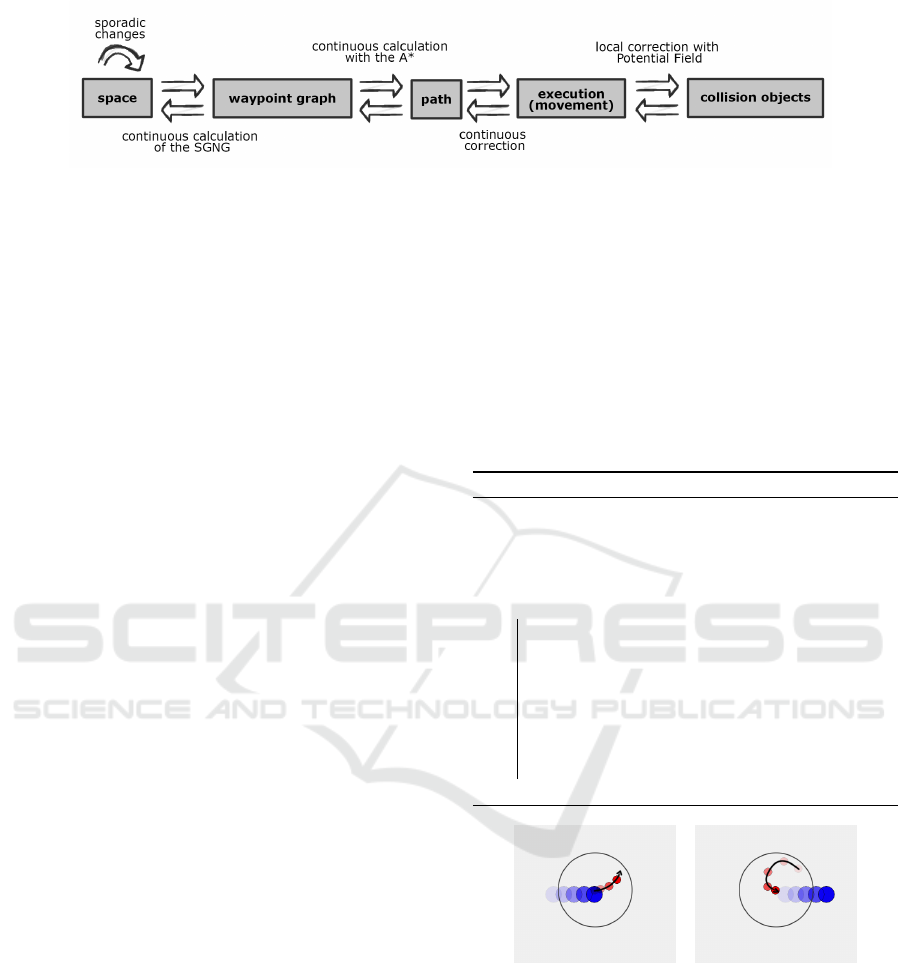
Figure 2: Structure of the NGDPP.

mostly in motion and it is usually much smaller than

the sporadic changes that might occur to the space. As

the neuronal gas takes some time to adapt to changes,

it is not practical to apply it directly to small fast mov-

ing objects. The much more important reason is, that

the graph should represent a globally valid topology

of the space. If we assume an area in which two

agents are to move independently, from an agent’s

point of view, the other agent is nothing more than

a collision object that moves relatively unpredictable.

If we applied the neural gas directly to avoid colli-

sion objects, it would be necessary to create a separate

SGNG graph for each individual agent as the graph

would no longer be globally valid. However, a glob-

ally valid graph yields the great advantage that it can

be calculated by one central processing unit, while it

can be used by multiple agents concurrently.

Therefore, we use the potential ﬁeld approach

(Koren and Borenstein, 1991) for collision objects. In

order to move several objects in the same space with-

out collisions, the phenomenon of electromagnetism

is copied from nature. It describes mathematically

the fact that two particles with the same charge re-

pel each other. This concept is applied to collision

objects. Objects within space are in principle treated

like particles with the same charge, so that in the event

of an impending collision they are repeled from each

other and thus prevent a collision.

On its own, the potential ﬁeld is not enough for

planning the route. However, it is very effective at

avoiding collisions between objects in local space.

Therefore it is used in our NGDPP algorithm. In or-

der to apply the “Potential Field” and allow an agent

to leave its planned path locally, we extend the ba-

sic agent which was only deﬁned by its position to a

“force ﬁeld agent” which is deﬁned by the three prop-

erties position of the force ﬁeld, detection radius and

position of the agent.

The agent is surrounded by a force ﬁeld within

which collision objects are detected. As a result, the

agent no longer has an absolute position in space, but

receives relative coordinates to the center of its force

ﬁeld. So instead of moving the agent directly along

its path, now the agent’s force ﬁeld is moved along

the path, with the agent normally located in the center

of the force ﬁeld (x = 0,y = 0). If a collision with

another agent is imminent, so if one enters the agent’s

force ﬁeld radius, the agent can move within its force

ﬁeld (see Figure 3). Because an attracting force is

constantly applied to the agent towards the center of

the force ﬁeld, the agent returns to its relative zero

position when no collision object is within its detec-

tion radius. Some more insight in the movement of

the agent is given in algorithm 2. The entire NGDPP

process is summarized in Figure 2.

Algorithm 2: agent.STEP( ).

Precon.:graph ← GRAPH(nodes ← [], edges ← [])

area ← LOADINITIALAREA()

collisionObjs ← LOADCOLLISIONOBJS()

target ∈ graph.nodes

1: function STEP(area, collisionObjs, graph)()

2: # move agent according to Section 3.3

3: MOVEAGENTINFORCEFIELD(collisionObjs)

4: # ﬁnd nearest node in the graph to s

5: n ← NEARESTNODE(agent.position, graph)

6: path ← PATHPLANNING(n, target)

7: # execute one step of the path

8: MOVEFORCEFIELD(path)

9: end function

(a) • (b) •

Figure 3: An agent (red) evades a collision object (blue)

within its force ﬁeld. After the collision object leaves the

detection radius, the agent returns to the center.

4 EVALUATION

In this section we will empirically evaluate the as-

sumption about the evenly distributed edge lengths

that we proposed and other properties of NGDPP, like

occurring collisions. Also, NGDPP is compared to

related work methods.

ICAART 2019 - 11th International Conference on Agents and Artiﬁcial Intelligence

142

4.1 Simpliﬁcation for the Usage of A*

In Section 3.2 the assumption was made, that the

SGNG algorithm produces a graph with equal-sized

edges. This simpliﬁes the path planning as the real

edge lengths do not have to be calculated, which

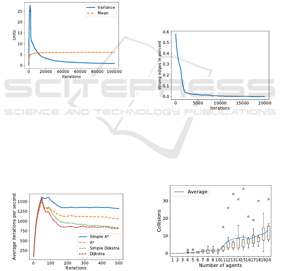
yields a performance advantage. In Figure 4 both

the mean values and the variances of the edge lengths

over 100,000 iterations are shown. There is a strong

rash in the variance at the beginning, but it converges

quickly towards zero. Also the mean value converges

against a certain value after a few thousand iterations

of the algorithm. That means, that it is sensible to

assume all edge lengths to be the same, i.e. to be one.

Figure 4: Mean and variance of all actual edge lengths over

more than 100,000 iterations of NGDPP.

The above assumption was used to compare the

performance of four different path planning algo-

rithms. Figure 5 shows, that the “simple” procedures,

which utilize the assumption, dominate the others in

terms of performance. In addition, it was checked for

more than 1 million iterations whether the methods

calculate a different path length. This could theo-

retically happen due to inaccurate edge lengths, but

also due to the heuristic mode of operation of the A*.

However, not a single deviation in the length of the

path was found. Not only does this improve perfor-

mance, it is also highly likely that the calculated path

Figure 5: Performance comparison of path planning algo-

rithms with and without the assumed simpliﬁcation.

will retain its quality.

4.2 Collisions

NGDPP is a heuristic algorithm and Collisions can

occur between agents as well as between agents and

their environment.

As mentioned in Section 3.1 the discretization of

the environment with SGNG is not perfect as the pre-

cision is bound to parameters of the algorithm and

also due to the fact that it iteratively adapts to changes

in the environment. That is why we measured the

number of wrong edges, that means, edges that in-

tersect with the environment (see Figure 1), after a

change of the map over time. The experiment shows

that the proportion for wrong edges (or nodes) de-

creases signiﬁcantly over time after a map change

(Figure 6).

Figure 6: Percentage of wrong edges over time.

Figure 7 shows the evaluation of occurring colli-

sions between agents. A number of 1-20 agents col-

lected random targets over 100,000 iterations in a free

space. Since collisions are probabilistic, the exper-

iment was repeated eight times for each number of

agents. The curve shows the average number of col-

lision per agent amount. It can be seen that a larger

number of agents leads more frequently to collisions.

Figure 7: Evaluation of the collision of multiple agents.

Dynamic Path Planning with Stable Growing Neural Gas

143

4.3 Comparison with Other Methods

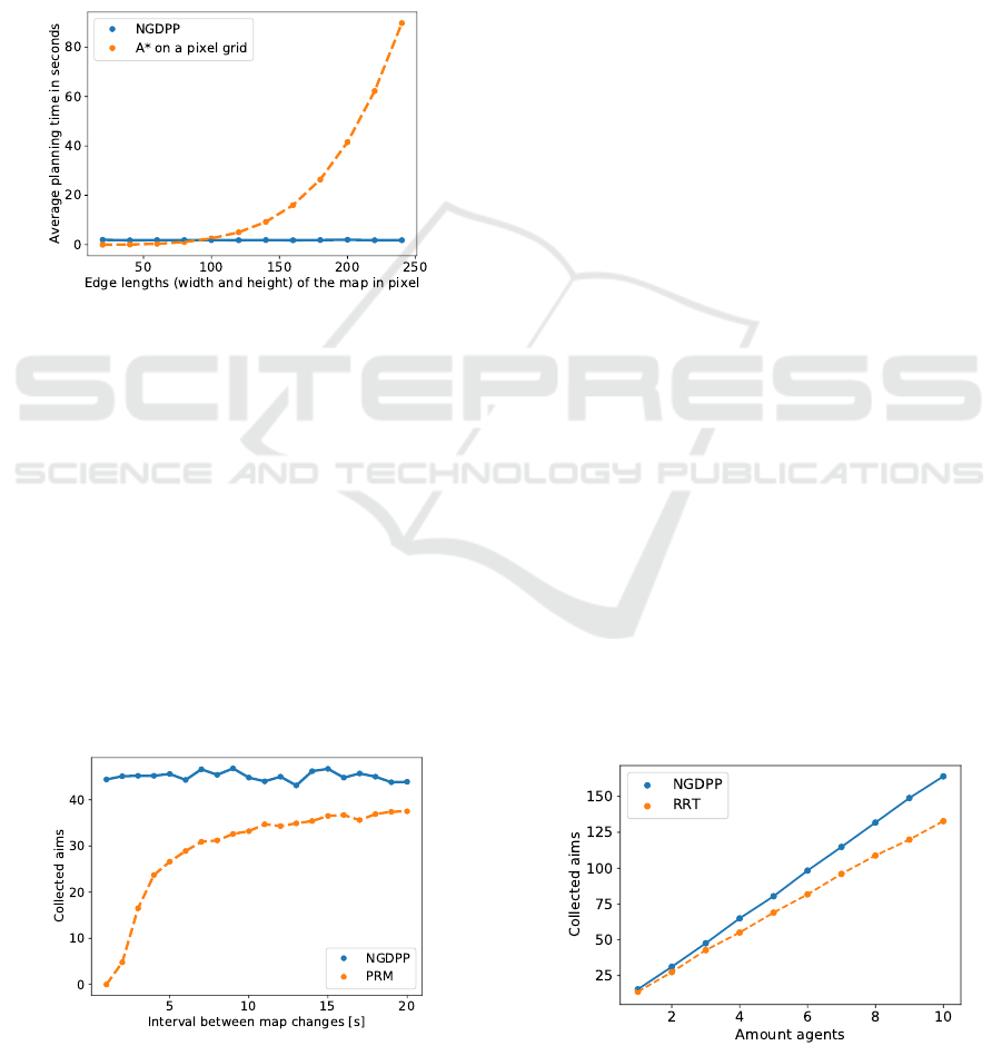
In Figure 8 the NGDPP algorithm is compared with

another, very simple pathﬁnding procedure to show

its efﬁciency. The method used for comparison uti-

lizes the A* algorithm for path ﬁnding, however, the

underlying graph results from the fact, that every

walkable pixel of the spatial plan is transformed into a

node, with edges between adjacent nodes. With larger

spaces, the runtime of this method increases quadrat-

ically while the NGDPP algorithm increases linear.

Figure 8: Performance comparison of NGDPP to A* rout-

ing on a graph that results from interpreting every pixel of

the input ﬂoor plan as node.

Comparison with PRM

In Section 2 the PRM approach was mentioned with

the point of criticism that the Probabilistic Roadmap

has to be completely rebuild after every change in

the space. During this reconstruction of the waypoint

graph no routing can be executed. In comparison, our

NGDPP approach dynamically adapts to changes and

continuously allows routing queries (with the restric-

tion that edges might collide with obstacles during the

adaption of changes and with inappropriate parameter

settings as mentioned in Section 3.1).

Figure 9: Performance comparison of NGDPP to a simple

PRM implementation (adapted from (Sakai et al., 2018)).

In the experiment both approaches were used for

the navigation of a single agent which had to collect

targets, that were spawned at random positions on the

map over the course of 5 minutes. In those 5 minutes

changes of the map occurred at different rates. The

changes had the character, that parts of the map be-

came accessible and were blocked again. The exper-

iment was repeated 10 times for each algorithm and

map change rate. The mean of the results is plotted in

Figure 9.

The results show that the agent using NGDPP col-

lects an almost constant amount of targets over the

course of 5 minutes as the adaption of the waypoint

graph to map changes and the path planning of the

agent are interleaved. On the other hand the agent us-

ing the PRM approach has to wait for the completion

of the waypoint graph before navigation can start. If

the interval between map changes is low, for example

2 second, the generation of the graph takes up most of

the time, leaving the agent no time to move before the

next change occurs and the graph as to be recreated.

Comparison with RRT

As mentioned in Section 2, one problem with RRT, a

method often used for path planning, is that a separate

graph (tree) has to be created for each agent. The con-

sideration here was that with an increasing number of

agents our method (NGDPP) should be superior to the

RRT method. This is based on the fact that in our case

all agents can use the same waypoint graph. In order

to verify this thesis empirically, we have carried out

an experiment.

We have used the two algorithms to let a number

of 1 - 10 agents collect randomly placed targets (but

the same for both) for 3 minutes in 10 different envi-

ronments. The results of this experiment can be seen

in Figure 10.

The experiment shows that the NGDPP is superior

to the RRT approach. Agents using NGDPP collect

more targets in the same time which is attributable to

Figure 10: Performance comparison of NGDPP to a simple

RRT implementation (adapted from (Sakai et al., 2018)).

ICAART 2019 - 11th International Conference on Agents and Artiﬁcial Intelligence

144

the higher planning time of RRT while the NGDPP

waypoint graph can continuously be used. This dif-

ference increases, as already assumed, with a higher

number of agents.

5 CONCLUSION AND FUTURE

WORK

In this paper, a new holistic method for path planning

in dynamic environments was presented: the NGDPP

algorithm. The sub problems of the problem domain

mentioned in the introduction, discretization, path

planning and collision avoidance, were dealt with sep-

arately. The dynamic discretization of the space was

solved using the SGNG algorithm. The resulting way-

point graph could then be used by the A* algorithm

to plan a valid path. During execution, this path is

locally adjusted using the “Potential Field” method,

so that collisions with dynamic obstacles are avoided.

Section 3 explains how these methods work together

to form the new NGDPP algorithm and which syner-

gies arise by the combination of them. In the evalua-

tion, the proposed changes that can be made to meth-

ods for the subproblems in order to obtain compu-

tational advantages, particularly the observation that

the used SGNG algorithm produces edges of equal

length, which accelerates the path planning, yield the

anticipated performance improvements. Overall, the

algorithm shows good performance compared to re-

lated work.

Up until now, our algorithm has only been applied

in simulations of holonome systems. However, most

real agents cannot take sudden turns through a 90

◦

an-

gle, for example. Such agents would probably not be

able to execute most paths planned by the NGDPP al-

gorithm. A possible solution for this could be smooth-

ing the path using Splines (Catmull and Rom, 1974)

respectively through the De-Casteljau algorithm (Alt

et al., 1997). To what extent this can be applied to

a path calculated by the NGDPP algorithm has to be

examined.

We assume, that our algorithm can be straightfor-

wardly adapted for three-dimensional spaces, since

all used methods, i.e. both neural gas and the “Po-

tential Field” as well as our proposed improvements,

would be possible in a three-dimensional application.

The algorithm could then be used e.g. for the move-

ment planning of ﬂying drones. However, the appli-

cability of our algorithm and its performance in three-

dimensional spaces has not been tested and leaves

room for further investigation.

REFERENCES

Alt, H., Welz, E., and Wolfers, B. (1997). Piecewise lin-

ear approximation of b

ezier-curves. In Proceedings

of the thirteenth annual symposium on Computational

geometry, pages 433–435. ACM.

Belghith, K., Kabanza, F., Hartman, L., and Nkambou, R.

(2006). Anytime dynamic path-planning with ﬂex-

ible probabilistic roadmaps. In IEEE International

Conference on Robotics and Automation, 2006. ICRA

2006., pages 2372–2377. IEEE.

Bentley, J. L. (1975). Multidimensional binary search

trees used for associative searching. Commun. ACM,

18(9):509–517.

Catmull, E. and Rom, R. (1974). A class of local interpo-

lating splines. In Computer aided geometric design,

pages 317–326. Elsevier.

Dellinger, B., Jenkins, R., and Walton, J. (2017). Auto-

mated waypoint generation with the growing neural

gas algorithm.

Dijkstra, E. W. (1959). A note on two problems in connex-

ion with graphs. Numerische mathematik, 1(1):269–

271.

Fritzke, B. (1995). A growing neural gas network learns

topologies. In Advances in neural information pro-

cessing systems, pages 625–632.

Hart, P. E., Nilsson, N. J., and Raphael, B. (1968). A for-

mal basis for the heuristic determination of minimum

cost paths. IEEE transactions on Systems Science and

Cybernetics, 4(2):100–107.

Kavraki, L. E., Svestka, P., Latombe, J.-C., and Overmars,

M. H. (1996). Probabilistic roadmaps for path plan-

ning in high-dimensional conﬁguration spaces. IEEE

transactions on Robotics and Automation, 12(4):566–

580.

Koren, Y. and Borenstein, J. (1991). Potential ﬁeld methods

and their inherent limitations for mobile robot naviga-

tion. In IEEE International Conference on Robotics

and Automation, 1991. Proceedings., pages 1398–

1404. IEEE.

LaValle, S. M. (1998). Rapidly-exploring random trees: A

new tool for path planning.

Legendre, P., Lapointe, F.-J., and Casgrain, P. (1994). Mod-

eling brain evolution from behavior: a permutational

regression approach. Evolution, 48(5):1487–1499.

Likhachev, M., Ferguson, D. I., Gordon, G. J., Stentz, A.,

and Thrun, S. (2005). Anytime dynamic a*: An any-

time, replanning algorithm. In ICAPS, pages 262–271.

Martinetz, T., Schulten, K., et al. (1991). A ”neural-gas”

network learns topologies.

Sakai, A., Ingram, D., Dinius, J., Chawla, K., Rafﬁn, A.,

and Paques, A. (2018). Pythonrobotics: a python code

collection of robotics algorithms.

Tenc

e, F., Gaubert, L., Soler, J., De Loor, P., and Buche,

C. (2013). Stable growing neural gas: A topology

learning algorithm based on player tracking in video

games. Applied Soft Computing, 13(10):4174–4184.

Dynamic Path Planning with Stable Growing Neural Gas

145