Wide and Deep Reinforcement Learning for Grid-based Action Games
Juan M. Montoya and Christian Borgelt
Chair for Bioinformatics and Information Mining, University of Konstanz, Germany
Keywords:
Wide and Deep Reinforcement Learning, Wide Deep Q-Networks, Value Function Approximation, Rein-
forcement Learning Agents.
Abstract:
For the last decade Deep Reinforcement Learning has undergone exponential development; however, less has
been done to integrate linear methods into it. Our Wide and Deep Reinforcement Learning framework provides
a tool that combines linear and non-linear methods into one. For practical implementations, our framework can
help integrate expert knowledge while improving the performance of existing Deep Reinforcement Learning
algorithms. Our research aims to generate a simple practical framework to extend such algorithms. To test
this framework we develop an extension of the popular Deep Q-Networks algorithm, which we name Wide
Deep Q-Networks. We analyze its performance compared to Deep Q-Networks and Linear Agents, as well as
human players. We apply our new algorithm to Berkley’s Pac-Man environment. Our algorithm considerably
outperforms Deep Q-Networks’ both in terms of learning speed and ultimate performance showing its potential
for boosting existing algorithms.
1 INTRODUCTION
In Artificial Intelligence there is an interest in cre-
ating rational agents which “act so as to achieve the
best outcome or, when there is uncertainty, the best-
expected outcome”(Russell and Norvig, 2003, p. 6).
The reinforcement learning (RL) problem seeks to
develop rational agents that learn from their environ-
ment by searching to maximize their outcomes using
a rewards system. These RL agents can accomplish
different kinds of tasks such as autonomous driving
(Kim et al., 2004), playing games (Mnih et al., 2015)
and directing robots (Kalashnikov et al., 2018). Since
the last decade, RL has been developing exponen-
tially, especially in the area of Deep Reinforcement
Learning (DRL) (Henderson et al., 2018).
Some examples of RL agents worthy of mention
that have used linear and non-linear functions to im-
prove and extend the RL framework. The autonomous
helicopter (Kim et al., 2004) from Standford Univer-
sity is an early work, where the agent learns to hover
in place and to fly a number of maneuvers by ap-
plying RL via Linear Function Approximation. This
implementation is efficient in training, as well as re-
solves and generalizes the problem of flying and hov-
ering. Nevertheless, it also assumes implicitly that
the problem is linearly solvable and so has limited
use in many (non-linear) real-world problems. In
2015, Deep Mind’s algorithm enabled RL agents to
successfully play 49 Atari games using a single al-
gorithm, fixed hyperparameters, and deep learning
(Mnih et al., 2015). Most recently, RL agents that
control robotic arms learn by applying similar princi-
ples how to generalize from their grasping strategies
so as to respond dynamically to disturbances and per-
turbations (Kalashnikov et al., 2018). Those network
architectures are robust and able to adapt to many
real-world problems; nevertheless, they inherit the al-
ready well-known difficulties of choosing and train-
ing neural networks and also require a lot of compu-
tation power (Goodfellow et al., 2016).
Researchers have been developing and treating
Linear Function Approximation and deep learning
separately to the best of our knowledge. Why not
combine wide learning (e.g. Linear Function Ap-
proximation) and deep learning to improve the per-
formance of RL algorithms? Fortunately, a wide and
deep machine learning framework has already been
developed in the field of recommendation systems
(Cheng et al., 2016). Our research aims to develop
a framework to transfer this approach to RL, making
it easy for researchers to extend already existing DRL
algorithms. To test our framework we developed an
extension of the popular Deep Q-Networks (DQN)
algorithm, which we name Wide Deep Q-Networks
(WDQN). We evaluated WDQN using a grid-based
50
Montoya, J. and Borgelt, C.
Wide and Deep Reinforcement Learning for Grid-based Action Games.
DOI: 10.5220/0007313200500059
In Proceedings of the 11th International Conference on Agents and Artificial Intelligence (ICAART 2019), pages 50-59
ISBN: 978-989-758-350-6
Copyright
c
 2019 by SCITEPRESS – Science and Technology Publications, Lda. All rights reserved

action game: Berkley’s Pac-Man environment. We
used Berkley’s Pac-Man environment because it is
highly scalable and computationally efficient. Fur-
thermore, solving the problem of playing Pac-Man is
not trivial. The DQN’s results on this game are some
of the worst among the 49 ATARI games, underper-
forming humans (Mnih et al., 2015).
Using the simple idea of combining both learning
approaches, we demonstrate that our WDQN trained
agent has a significantly higher winning rate and pro-
duces much better results compared to solely linear or
non-linear agents, and has better learning speed com-
pared to DQN.
Our research is now divided into six sections. In
the “Background” section we do a review of Linear
Function Approximation and DQN and then present
our theoretical framework “Wide and Reinforcement
Learning”, which we used to develop the WDQN
algorithm. In the section entitled “Experiments”
we show how WDQN performs compared to DQN,
Linear Function Approximation, and humans. For
this, we expose how Berkley’s Pac-Man environment
works, the experimental set-up for WDQN, and the
results. Next, we discuss the results and then present
our conclusions.
2 BACKGROUND
2.1 Linear Function Approximation
RL agents receive feedback from their actions in the
form of rewards from interacting with the environ-
ment. The agents aim to resolve a sequential decision
problem by optimizing the cumulative future rewards
(Sutton and Barto, 2018). One of the most popular
methods to resolve this is Q-learning (Watkins, 1989;
Henderson et al., 2018). Nevertheless, Q-Learning
alone cannot compute all value functions when con-
fronted with a large state space, which is the case
for most real-world problems (Russell and Norvig,
2003).
One way of tackling the large state space problem
is to use a function
ˆ
Q to approximate the true q-value
Q. Differentiable methods, such as linear combina-
tion of features and neural networks, offer us the pos-
sibility of using stochastic gradient descent (SGD) as
an intuitive form to optimize the action value func-
tion.
The equation using a Q-learning update after tak-
ing action A
t
in state S
t
observing the immediate re-
wards R
t+1
and continuing state S
t+1
is then
θ
t+1
= θ
t
+ α(y
ˆq
t
−
ˆ
Q(S
t
, A
t
;θ
t
) 5
θ
t
ˆ
Q(S
t
, A
t
;θ
t
) (1)
where α is a scalar step size, θ
t
the parameters of
the function
ˆ
Q, and the target function y
ˆq
t
defined as
R
t+1
+ γ max
a
ˆ
Q(S
t+1
, a;θ
t
). Gradient descent is ap-
plied by optimizing a loss function from the differ-
ence of y
ˆq
t
and
ˆ
Q(S
t
, A
t
;θ
t
).
The value function can be approached us-
ing a linear combination of features f (S
t
) =
[ f
1
(S
t
), ..., f
n
(S
t
)]
t
. Each f
i
(S
t
) represents a feature
mapped at state S
t
with a particular function f
i
. The
q-value function is constructed as Q
LN
(S
t
, A
t
;θ
LN
t
) =
f (S
t
)
T
θ
LN
t
, where θ
LN
t
are the weights of the linear
function. The target is then defined as
y
LN
t
:= R
t+1
+ γ max
a
ˆ
Q
LN
(S
t+1
, a;
ˆ
θ
LN
t
) (2)
The differential of (1) applied to f (S
t
)
T
θ
LN
t
is
then θ
LN
t+1
= θ
LN
t
+α(y
LN
t
−Q
LN
(S
t
, A
t
;θ
LN
t
) f (S
t
). It is
therefore a simple matter to compute the update rule.
In practice, linear methods can be very efficient
in terms of both data and computation. Nevertheless,
prior domain knowledge is usually needed to create
useful features, representing interactions between fea-
tures can be difficult, and convergence guarantees are
limited to linear problems (Sutton and Barto, 2018).
2.2 Deep Q-Networks
The intuitive action to resolve non-linear cases is
to substitute the approximation function
ˆ
Q with a
non-linear function using neural networks. However,
this first “naive” approach underperformed because of
problems with non-stationary, non-independent, and
non-identically distributed data (Mnih et al., 2015).
The DQN tackle such problems by using an ex-
perience replay memory and target networks. DQN
use a convolutional neural network (convNets) archi-
tecture to compute the state S
t
to a vector of action
values. This q-value function is Q
DQN
(S
t
, A
t
;θ
DQN
),
where θ
DQN
are the parameters of the convNets. The
experience replay (Lin, 1992) saves observed transi-
tions for some time in a dequeue. These transitions
are later uniformly sampled and used to update θ
DQN
.
The parameters
ˆ
θ
DQN
of the target network
ˆ
Q
DQN
are
copied from the online network every τ steps, so that
ˆ
θ
DQN
= θ
DQN
, fixing
ˆ
θ
DQN
on all other steps. The
target used by DQN is then
y
DQN
t
:= R
t+1
+ γ max
a
ˆ
Q
DQN
(S
t+1
, a;
ˆ
θ
DQN
) (3)
Both components dramatically improve the perfor-
mance of the algorithm (Mnih et al., 2015) and have
been successfully extended since their creation (Hen-
derson et al., 2018). However, DQN and variants in-
herit all the problems related to neural networks such
as the difficulty of interpreting the decision making
Wide and Deep Reinforcement Learning for Grid-based Action Games
51

Features
DeepComponent
a
2
a
m
....
Dense
Layer
Convolutional
Layers
WideComponent
Action
Values
preprocessing
a
1
State
w
1
w
2
w
n
f
1
f
2
....
f
n
conv
1
conv
2
conv
k1
....
neuron
p
neuron
1
neuron
2
ŵ
11
ŵ
21
ŵ
p1
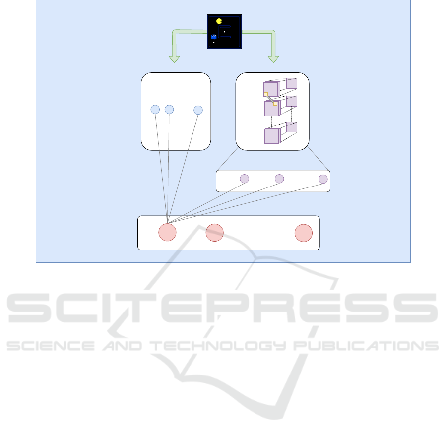
Figure 1: Wide and Deep Reinforcement Framework showing the connections from the weights of the deep and wide compo-
nent to action value a
1
.
of the networks, the tuning of multiple hyperparame-
ters (Goodfellow et al., 2016), and the complexity in
computation with no guarantees of convergence (Sut-
ton and Barto, 2018).
Our approach proposes to combine both linear and
non-linear methods in order to obtain better, faster and
more comprehensive results using DQN Algorithms.
Cheng et al. (2016) already showed that such a wide
deep learning model is viable and significantly im-
proves the results for recommendation systems.
3 WIDE AND DEEP
REINFORCEMENT LEARNING
Figure 1 shows the general structure of the Wide and
Deep Reinforcement Learning (WDRL) Framework,
which can be used for already existing DRL algo-
rithms. This framework consists of the linear combi-
nation of features (left side) and convNets (right side),
which are respectively called the wide and deep com-
ponent. Both components compute the action values
A = [a
1
, ..., a
m
].
Initially, the states are preprocessed separately for
the wide and deep component. For this step, the pre-
processing function φ needs to be able to process the
state S
t
separately for the wide and the deep com-
ponent. The state S
t
needs to be processed indepen-
dently for each component because the inputs are dif-
ferent for each component. The wide component re-
quires information provided by the features, while the
deep component takes an image representation to be
processed by the convNets in our case.
3.1 The Wide and Deep Component
In Figure 1, the wide component uses a linear combi-
nation of features f
1
, ..., f
n
, which are connected with
their respectively weights θ
LN
= [w
1
, ..., w
n
]
t
to each
value action a
i
of the approximation functions. In
this illustration, we represent the weights as shared
weights (e.g. as a vector) because they correspond to
the implementation used in our experiments. The fea-
tures can be represented by a feature matrix F ∈ R
m,n
,
where m is the total number of outputs and n the num-
ber of features. Figure 1 shows [F
1,1
, ..., F
1,n
] = F
1n
multiplied by θ
LN
for a
1
. The optimization step can
be easily inferred from (1).
In our illustration, the deep component uses
the convNets [conv
1
, conv
2
, ..., conv
k−1
] for almost
all layers. Each hidden layer except for the last
one performs the following computation a
(l+1)
=
ˆ
f (
ˆ
W
(l)
a
(l)
+ b
(l)
), where l is the layer number and
ˆ
f is the activation function, a
(l)
, b
(l)
, and
ˆ
W
(l)
are
the activations, bias, and function weights at the l·-
·th layer. The last layer k implements a dense layer,
ICAART 2019 - 11th International Conference on Agents and Artificial Intelligence
52

but it could also be extended to have more fully con-
nected layers. In addition, this final layer does not use
an activation function so that a
(k)
=
ˆ
W a
(k−1)
+b
(k−1)
,
where
ˆ
W
(k−1)
=
ˆ
W ∈ R
pm
. Figure 1 shows also that
a
(k−1)
= [neuron
1
, ..., neuron
p
]
t
and the weights of the
last layer for a
1
are represented by [ ˆw
11
, ..., ˆw
p1
]
t
=
ˆ
W
p1
.
The wide and deep components are combined to
generate the output of the Wide and Deep Reinforce-
ment function. Figure 1 shows that a
1
= F
1,1
· w
1
+
... + F
1,n
· w
n
+ neuron
1
·
ˆ
W
1,1
+ neuron
1
·
ˆ
W
1,1
+ ... +
neuron
p
·
ˆ
W
p,1
, which is equal to a
1
= F
1n
· θ
LN
+
a
( f −1)
·
ˆ
W
p1
. This can be easy generalized to all action
values: A = F · θ
LN
+ a
(k)
.
Now, in order to train the function, two ap-
proaches can be implemented. The first approach
is called joint ensemble training and computes SGD
jointly for the linear and non-linear functions. We
call the second approach semi-ensemble training be-
cause, in contrast to ensemble training in supervised
machine learning, predictions of the linear and non-
linear functions do influence each other during train-
ing (Cheng et al., 2016). However, as in ensemble
training, this approach implements SGD separately
for both functions. Both approaches use the combined
prediction of the linear and non-linear function to act.
3.2 Wide Deep Q-Networks
The DQN Algorithms can be extended by integrat-
ing the linear function Q
LN
with the non-linear func-
tion Q
DQN
creating the combined function Q
W D
; thus
called “Wide Deep Q-Networks”.
For our illustration using WDQN, the wide com-
ponent uses the target function for the linear combi-
nation of features shown in (2). Meanwhile, the deep
component uses the target function of (3). There-
fore, the combined function is Q
W D
(S
t
, A
t
;θ
W D
) =
Q
LN
(S
t
, A
t
;θ
LN
) + Q
DQN
(S
t
, A
t
;θ
DQN
), where θ
W D
includes the parameters of the wide and deep func-
tion.
For the joint training, the algorithm remains al-
most identical to the original DQN. The online Q
DQN
and target network
ˆ
Q
DQN
need only be replaced by
Q
W D
and
ˆ
Q
W D
respectively. The target is then defined
as
y
W D
t
:= R
t+1
+ γ max
a
ˆ
Q
W D
(S
t+1
, a;
ˆ
θ
W D
) (4)
where
ˆ
θ
W D
are the target parameters of the combined
function. The SGD is estimated directly on the joint
function.
For the semi-ensemble training, the algorithm
needs to save the linear and non-linear function, as
Algorithm 1: Semi-Ensemble Training WDQN.
1: Initialize:replay memory D to size N;
2: Action-value functions Q
W D
, Q
LN
, Q
DQN
with
respectively random weights θ
W D
, θ
LN
, θ
DQN
;
3: Target action-value functions
ˆ
Q
W D
,
ˆ
Q
LN
,
ˆ
Q
DQN
with weights
ˆ
θ
W D
= θ
W D
,
ˆ
θ
LN
= θ
LN
,
ˆ
θ
DQN
= θ
DQN
respectively.
4: for episode = 1, M do
5: Initialize sequence S
1
= [x
1
]
6: Preprocessed sequence φ
1
= φ(s
1
)
7: for t = 1,T do
8: With probability ε select a random action
a
t
∈ A
t
otherwise select:
a
t
= argmax
a
Q
W D
(φ(s
1
), a; θ
W D
)
9: Execute action a
t
, observe
reward R
t
and image x
t+1
10: Set S
t+1
= S
t
, a
t
, x
t+1
and preprocess
φ
t+1
= φ(S
t+1
)
11: Store transition (φ
t
, a
t
, R
t
, φ
t+1
) in D
12: Sample random minibatch of transitions
(φ
t
, a
t
, R
t
, φ
t+1
) from D
13: Set y
DQN
j
, y
LN
= r
j
for terminal φ(S
j+1
)
and non terminal φ(S
j+1
):
y
DQN
j
= R
t+1
+ γmax
a
ˆ
Q
DQN
(S
t+1
, a;
ˆ
θ
W D
)
y
LN
j
= R
t+1
+ γmax
a
ˆ
Q
LN
(S
t+1
, a;
ˆ
θ
LN
)
14: Perform gradient descent on
(y
DQN
j
− Q(S
t+1
, a; θ
DQN
))
2
and
(y
LN
j
− Q(S
t+1
, a; θ
LN
))
2
with respect to θ
LN
and θ
DQN
15: Every C steps reset
ˆ
θ
LN
= θ
LN
,
ˆ
θ
W D
= θ
W D
and
ˆ
θ
DQN
= θ
DQN
.
16: end for
17: end for
well as the combined function (see Algorithm 1). Ba-
sically, the actions are being chosen by the combined
function Q
W D
, however SGDs are estimated sepa-
rately on Q
LN
and Q
DQN
, implementing both targets
from (2) and (3).
4 EXPERIMENTS
4.1 The Pac-Man Environment
In order to compare the different algorithms with each
other, we used the Pac-Man open source environment
of UC Berkeley (DeNero and Klein, 2010). Our goal
was not to use a fully realistic simulator of Pac-Man
to achieve superhuman results, but rather to have a
scalable and computer efficient environment to test
our Deep and Wide Reinforcement framework. The
Pac-Man environment of UC Berkeley is suitable for
this: the scalability is guaranteed by providing cus-
tomizable map sizes. Moreover, the preprocessing of
the game states is more efficient than using raw pixels
Wide and Deep Reinforcement Learning for Grid-based Action Games
53

(more details coming below). We decided to test our
approach only on small and medium maps due to our
computational limitation of one 12 GB NVIDIA Ti-
tan GPU. We analyzed the performance of our agents
for each map. We have chosen ConvNets because
they share weights across maze positions creating in-
dependence between maze locations and accelerat-
ing training speed. This is an advantage compared
to fully connected nets with the same amount of lay-
ers (Goodfellow et al., 2016), reassuringly, the use of
ConvNets has been a standard tool for DRL research
(Mnih et al., 2015; van Hasselt et al., 2016; Hender-
son et al., 2018).
For a more complex and fully realistic Pac-Man
environment see Ms. Pacman used in (Mnih et al.,
2015; van Hasselt et al., 2016). In order to guaran-
tee transparency and reproducibility, our Python code
using Tensorflow is available at GitHub
1
. We follow
the recommendations of Henderson et al. (2018) to
include the used hyperparameters and random seeds.
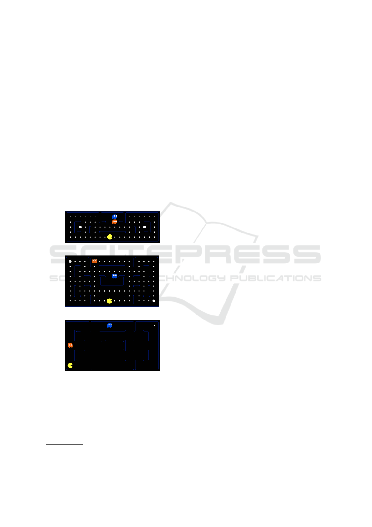
(a)
(b)
(c)
Figure 2: The small (a) and medium (b) maps of Berkeley’s
Pac-Man environment at the agent’s starting point. The
medium map in (c) shows the last dot that has to be eaten in
order to finish the game.
Figure 2 shows our implemented maps in Berke-
ley’s Pac-Man environment. Pac-Man, the yellow
agent, can move vertically and horizontally, eating
dots on his way. The goal of Pac-Man is to score as
1
https://github.com/JuanMMontoya/WDRL
many points as possible by eating the small dots all
around the maze while avoiding crashing into any of
the ghosts that are chasing him. Additional points are
given if Pac-man eats the special edible ghosts. The
ghost becomes temporally edible when Pac-Man eats
one of the big dots on the board. Eaten ghosts reap-
pear back as not edible ghosts. An episode is finished
when Pac-Man either eats the last dot (see (c) in Fig-
ure 2) or gets killed by a non-edible ghost.
In both maps, Pac-Man starts in the top middle
part of the map which also contains two ghosts, many
small dots, and two big dots (see (a) and (b) in Fig-
ure 2). The room, where the ghosts start and reap-
pear if they get killed, is in the middle of the maze for
medium map and at the top of the maze for the small
map. For scoring, we used the original reward system
of UC Berkeley. The initial score is always zero and
restarts after each episode. Eating the small and big
dots scores 10 points. For each eaten edible ghosts,
the agent scores 50 points. In order to avoid stagna-
tion, the agent is deducted 1 point for each second
that is spent. At the end of an episode, Pac-Man ei-
ther wins, scoring 100 points or loses, deducting 500
points.
A profitable approach to achieve higher scores is
to eat ghosts because of the high rewards. Neverthe-
less, the original DQN algorithm did not learn to eat
them (Mnih et al., 2015), explaining to some extent
the poor scores of DQN in this game. Their DQN
agent received a clipped reward of either 1 or -1 at
each state S
t
. For example, the agent gets 1 point for
eating either a ghost or a dot; a negative score, for
dying, is -1. The agent, therefore, did not learn the
significance of eating ghosts because of the low re-
ward (van Hasselt et al., 2016). However, the agent
did learn to eat ghosts in two other approaches: Has-
selt et al. (2016) confronted this problem by adap-
tively normalizing the targets of the network, making
it possible to process all types of rewards. Meanwhile,
Van der Ouderaa (2016) used the incoming reward of
Berkeley’s environment at each state S
t
to train the
DQN algorithm.
For our approach, we preferred to use Van der
Ouderaa’s method, because it keeps our implementa-
tion as minimalistic as possible and was also tested
using the same reward system. In addition, in our
experiments, we decided to distinguish whether the
trained agents can or cannot eat ghosts. We consider
that an agent can only eat a ghost when it actively
hunts the edible ghost and not purely by chance. To
do this, we observed at least 10 games for each of the
selected agents.
In order to save computational power, raw pixels
are not used as the input for the deep component (also
ICAART 2019 - 11th International Conference on Agents and Artificial Intelligence
54

for DQN). For agents that learn directly from pix-
els see (Mnih et al., 2015; van Hasselt et al., 2016).
The input we implemented, consists of an array with
six matrices containing the coordinates respectively
of each 1) ghost, 2) wall, 3) dot, 4) big dot, 5) Pac-
Man and 6) edible ghost (van der Ouderaa, 2016). In
each matrix, a 0 or 1 respectively expresses the ex-
istence or absence of the element at each coordinate
on its corresponding matrix. These matrices are eas-
ily retrievable for each state and they are a distinctive
quality of using Berkeley’s environment.
The matrix size is defined by the width W and
height H of the game grid. The input, therefore, has
the following dimensions of W × H × 6. This per-
mits a fast identification of the important game ele-
ments. In combination with the size favorable maps,
the inputs’ preprocessing and the back-propagation
are computed efficiently.
For the wide component, we used the Linear
Function Approximation contained in the Berkeley
environment. This consist of the three features struc-
tured in the following way:
1. #-of-ghosts-1-step-away: lets the agent know the
number of ghosts one step away and does not dif-
ferentiate between edible and non-edible ghosts.
2. eats-food: sets to one if there is a ghost one step
away and zero if there isn’t.
3. closest-food: gives the direction to the closest dot.
Notably, the linear agent cannot eat ghosts. We
found that the main reason for such a behavior is the
inability of #-of-ghosts-1-step-away to distinguish the
ghost type. This creates a dichotomy: either learning
to eat ghost or avoiding them. Since the reward incen-
tives are higher to survive he chooses to evade them.
4.2 Experimental Set-up
The algorithms analyzed are the Linear Function Ap-
proximation, DQN, and WDQN. To tune the hyper-
parameters we performed around 100 preliminary ex-
periments for the linear and DQN agent in differ-
ent maps. We adjusted mainly the size of the mem-
ory replay, the learning rates, the update rate of the
target function, the network structure, and the ex-
ploration value ε with its final exploration frame.
We consistently maintained the final hyperparameters
shared between the linear and DQN agent. Afterward,
we used these hyperparameters for the WDQN. All
agents also have also the same action values, i.e. four
possible directions: left, right, up, down.
In addition, we found that the learning curve stag-
nated around 10000 episodes. Therefore, we have
chosen this value as the training limit for the final
experiments. In order to compare the agent’s per-
formance against each other, we decided to use the
averaged score and the win rate of each agent for
100 episodes. Finally, we repeated multiple random
seeded experiments with the same hyperparameters
for each selected agent to guarantee consistency.
Our DQN-agent do not apply the same hyperpa-
rameters but rather the same algorithm structure de-
scribed in (Mnih et al., 2015). Our convNet has two
convolutional layers and one fully connected layer
that maps into the four outputs. The first layer applies
16 3× 3 filters with full padding and one stride, while
the second 32 3 × 3 filters with full padding and one
stride. The fully connected layer has 256 neurons.
The learning rate was set up to 0.001 using ADAM
optimization algorithm. This architecture permits us
to maintain the network small but with the capacity
of making complex decisions. By using height and
width 3x3 filters in two layers (resulting in a 5x5 field
of view) it permits the agent to see at least 2 steps
away from him. This is important for avoiding been
eaten. The two layers with a depth of 16 and 32 di-
mensions respectively allow the agent to be able to
abstract from a combination of 32 different base maze
patterns. A similar architecture was implemented in
(van der Ouderaa, 2016) and was confirmed during
our preliminary experiments.
Using the linear combination of features, the lin-
ear agent chooses the policy at state s
n
that could
give him the highest q-function at the next state s
n+1
.
The sequence of training for our linear approximator
follows the DQN’s algorithmic structure (i.e. target
function, memory replay, etc.). The learning rate was
set up to 0.1 using SGD. The exact description of the
applied hyperparameters for all agents can be found
in our GitHub’s repository.
The WDQN algorithm is trained using semi-
ensemble training because of the preliminary knowl-
edge of learning rates for the linear function and con-
vNets. The listed features of the last subsection are
implemented in the wide component using different
combinations of features. The WDQN algorithm is
tested separately using a wide component with three,
two, and one feature(s) respectively. We decided to
combine the features in the following way because:
1. Combining the three available features permits us
to mix DQN and the Linear Approximator com-
pletely.
2. By avoiding using the feature #-of-ghosts-1-step-
away, the two features closest-food and eats food
do not contain the strongest constraint to not learn
eating ghosts.
3. The feature #-of-ghosts-1-step-away should en-
able faster learning to win, because it gives the
Wide and Deep Reinforcement Learning for Grid-based Action Games
55

most important information on how to survive the
game.
Table 1: Score Average and Win rate in Small and Medium
Map, as well as whether the agents learned to eat ghosts.
The agents presented are the Linear Function Approxima-
tion, DQN and WDQN with 3, 2 and 1 features respectively,
as well as the Random agent. For each algorithm, the best
agent is chosen and evaluated for 100 episodes. The best
amateur human player also played 100 games.
Small Map Medium Map Eats
GhostsScore Win Rate Score Win Rate
Linear -108 18% 486 55% no
DQN 110 33% 622 47% yes
WDQN 3 feat. 296 60% 666 64% no
WDQN 2 feat. 353 61% 727 65% yes
WDQN 1 feat. 215 51% 614 61% no
Human -99 11% 125 12% yes
Random -463 0% -443 0% no
4.3 Results
Figure 3 shows the achieved scores for each agent in
the small (right side) and medium map (left side) dur-
ing training. A clear difference of training speeds is
observable between algorithms. The WDQN 3 and 2
features agents learn faster than the WDQN 1 feature
and the DQN agents. The linear agent learns faster
than all other agents but stabilizes once arriving at a
certain threshold, which is exceeded by all agents us-
ing neural networks at some point. The learning speed
also varies depending on the map.
In the medium map, we see that the training is
faster than in the small map. For instance, in the
medium map, the WDQN 3 and 2 features surpass the
score of the linear agent at 4000 episodes and DQN at
6700 episodes. This results in a difference of 2700
episodes between WDQN and DQN. Meanwhile, the
WDQN 3 and 2 features agents in the small map
reach the score of the linear agent at 3900 episodes,
while DQN at 5700 episodes. This is a difference of
1600 episodes. Thus, there is a substantial disparity
of training speed between WDQN and DQN agents,
which also varies depending on the map.
In addition, Figure 3 presents the different perfor-
mance of the algorithms during training. WDQN 3
and 2 features perform better than the WDQN 1 fea-
ture and DQN agents. The linear agent achieves the
worst results followed by WDQN 1 feature, while
DQN stays only behind the outcomes of WDQN 3
and 2 features. Yet again, there are notable differences
between maps. First, the WDQN 3 features agent be-
haves better in the small map than in the medium map.
Second, the performance gap between worst and bet-
ter agent is more unequivocal in the small than in the
medium map.
Table 1 shows the averaged score and winning rate
for WDQN, DQN, Random and Linear agents, and
human players in the small and medium map for 100
episodes. Table 1 illustrates that the WDQN 3 and
2 features have the best averaged score and win rate
among all agents, while the DQN agent is at 3
rd
or
4
th
place depending on the map. The best agent is
WDQN 2 features. The agent wins 61% with 353
points and 65% with 727 points respectively for the
small and medium map and learns to eat ghosts. At
the same time, the WDQN 3 features agent has a
slightly smaller win rate than WDQN 2 features but
scores lower than such an agent and cannot eat ghosts.
The DQN agent underperforms those agents and
learns to eat ghosts as shown in Table 1. However, in
the medium map, the difference in score to WDQN
3 and 2 features is less than 120 points, although the
DQN agent loses more than half of the games. In con-
trast, the linear agent wins a little more than half of the
games but scores around 120 points less than DQN.
As already stated, the linear agent cannot eat ghosts
because of the features being used. The WDQN 1
feature agent wins less than the other WDQN agents
and cannot eat ghosts. In the case of the medium map,
it scores lower than the DQN agent.
Furthermore, the results for our amateur human
players are below the non-random agents with around
11% of games won. The only slight exception is
the score (-99) against the linear agent in the small
map (-108). For the human row, we selected the best
players of a round-robin tournament with 9 volunteers
(see our GitHub repository for the recorded human’s
games ). This shows us that the problem is not triv-
ial for humans. Random agents have the worst results
(-463 and -443); thus, moving by chance is not a prof-
itable option for this game.
The Figure 3 and Table 1 present almost equiva-
lent outcome. Yet, the most notable contrast is that
the best agent during training is WDQN 3 features in
Figure 3 (left side), but the best scores in Table 1 are
produced by WDQN 2 features.
The present findings confirm that the WDQN
agent can perform better than DQN, linear and ran-
dom agent, as well as the amateur human players.
WDQN algorithm with 3 and 2 features have the best
score and win rates. In addition, they learn faster than
the DQN agent. Nevertheless, the WDQN 1 feature
agent has a lower score and learning speed than the
other WDQN’s. Our assumption that WDQN 1 fea-
ture could learn faster is proven to be wrong.
Lastly, we detect some tendencies in the results
that are worth examining more closely. There is a
learning speed difference between maps that could be
related to the performance of the linear agent. More-
ICAART 2019 - 11th International Conference on Agents and Artificial Intelligence
56

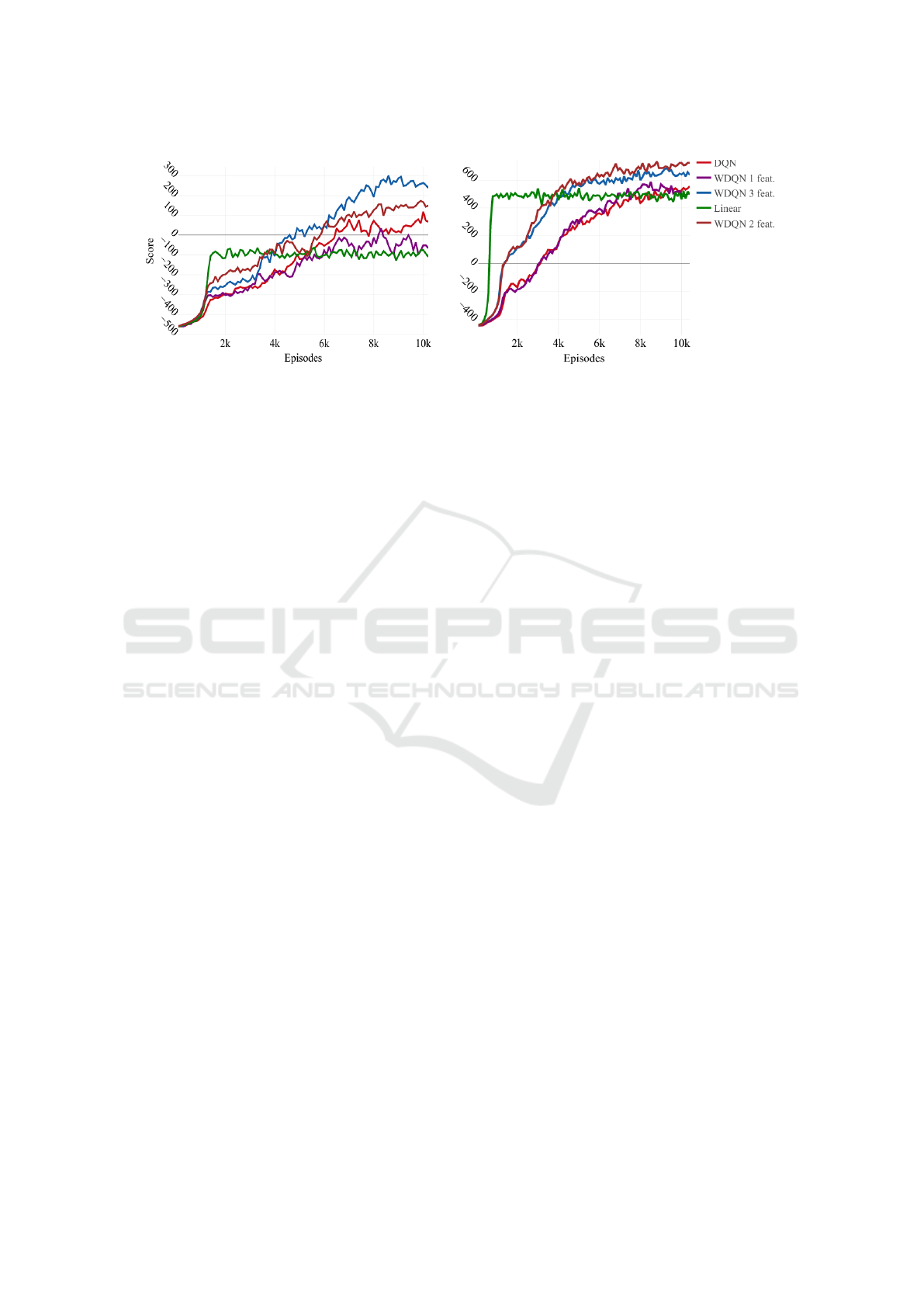
Figure 3: Each agents score is evaluated during training for the small (right side) and medium map (left side). Five random
seeded training sessions are conducted for each agent with the same hyperparameters until 10200 episodes respectively in the
small (a) and medium map(b). The lines arise of averaging those training sessions according to the agent type.
over, there are algorithms that learn to eat ghosts,
while others do not, depending on the implemented
feature. Finally, making only random moves is a
high unproductive strategy both to win and score high.
This could be part of a pattern that explains the nega-
tive results of the DQN agent.
5 DISCUSSION
The results presented confirm the better performance
of the combined WDQN agent compared to the solely
DQN and linear agent. Now, we concentrate on dis-
cussing the reasons for such improved performance
by analyzing the learning speed difference between
maps, why some agents eat ghosts or not, and the
logic behind the DQN’s underperforming.
For WDQN 2 and 3 features agents, we observe a
speedup of the learning during training results, which
depends on the map. The linear agent’s performance
can be the key to understand such a difference. In
the medium map, the linear agent works considerably
better than on the small map. The superior results of
the linear agent in the medium map influence those
WDQN agents to learn faster and more prolonged
than in the small map.
In addition, we observe that the poor results of the
linear agent are not transferred to the WDQN agents
in the small map. This could imply that our linear
function cannot abstract a proper solution to the game,
although the features itself provide valuable informa-
tion.
The scores and win rates of the trained agents
show that the WDQN agents with the #-of-ghosts-
1-step-away feature do not learn to eat ghosts. This
explain why the WDQN 2 features outperforms the
WDQN 3 features learns to eat ghosts scoring more.
Furthermore, by looking at WDQN 1 feature’s per-
formance, the #-of-ghosts-1-step-away feature helps
to develop the capacity to survive in short-term. Yet,
it restricts the capacity to achieve high scores in long
term.
We observed that the weights of the wide com-
ponent change faster and stronger than those of the
deep component because of its simple updates. In the
case of WDQN 3 feature, there is an information con-
flict between the deep component and the wide com-
ponent. The features of the linear component treat
all ghosts identically, while the input of deep compo-
nent can see the difference between edible and not.
From this conflict the wide component is more domi-
nant because of its weights. If there is no compensa-
tion of this effect, for example, by normalizing the
weights, switching on and off the wide component
during training or only training more episodes, we
suspect that WDQN agents using this feature will not
learn to eat ghosts.
Repetitive observations of the DQN agent’s play
leads us to detect that the agent had difficulties reach-
ing the last dots in the map. This was especially true
if the dots were far away from the agent. Figure 2
(c) illustrates exactly such a case, where the agent is
considerably far for the last dot. We believe that:
1. Reaching the last dot is complicated because the
reward propagation usually happens in a different
place each game.
2. Making random moves does not permit Pac-Man
to explore the map because the ghosts can easily
kill him when maneuvering randomly. Rather, the
DQN agent seems to reach far away dots thanks
to the movements caused by avoiding ghosts.
In both cases, there are insufficient examples to
learn how to detect the exact position of far away dots.
This could explain the success of the WDQN 3 and 2
features. The wide component adds the information
about where to find such dots.
Wide and Deep Reinforcement Learning for Grid-based Action Games
57

However, we should not exclude the possibility
that the DQN problems could be related to the chosen
hyperparameters, especially of the convNets. Maybe
choosing larger filters could contract such problem.
Moreover, assuming that the DQN has an excellent
solution in itself in another different implementation,
maybe adding a wide component would improve nei-
ther the training speed nor the results.
Conclusively, we believe that integrating a good
wide component to the WDQN model can be the rea-
son for a substantial speedup of learning. Adding a
deep component to a linear agent could improve its
linear limitation considerably by converting it into
a non-linear model. Precautions are needed when
choosing which features to integrate into the com-
bined agent. Lastly, a favorable wide component can
compensate for the difficulties of the deep component
to learn from insufficient examples.
6 CONCLUSION
Our research shows that the WDQN agents can out-
perform linear and DQN agents in score, winning rate
and learning speed. The chosen features also play a
role in achieving these results. However, there can
be learning limitations depending on the selected fea-
ture(s). The research demonstrates that combining a
neural network with a linear agent helps improve re-
sults by allowing the model to learn non-linear rela-
tionships while adding information about the interac-
tion between specific features, while also making the
agent adaptable to uncertainty. Furthermore, the wide
component can complement the weaknesses of a non-
linear agent by helping the agent learn faster and con-
centrate on finding less obvious important features.
Our method is straightforward and employable for
various deep reinforcement contexts. For real-world
implementations such as robotics, the combination of
linear and non-linear functions in our Wide and Deep
Reinforcement Learning provides an interesting tool
for integrating new devices like sensors in the form
of features into DRL agents, or for including better
expert knowledge with human chosen features. Fu-
ture work could look into extending WDQN to in-
clude newer DQN-related algorithms and developing
methods that make implementing WDQNs easier; for
example, automatically setting the learning rate of the
wide component from the deep component’s to re-
duce the number of hyperparameters. In addition, one
could research how to ensure that the influence of neg-
ative features of the wide component can be overrid-
den by the deep component.
ACKNOWLEDGEMENTS
We thank our colleagues from the Chair for Bioinfor-
matics and Information Mining of the University of
Konstanz, who provided insight and corrections that
greatly assisted the research. Especially, we are grate-
ful to Christoph Doell and Benjamin Koger for the
continuous assistance with the paper’s structure and
the engineering of the deep neural networks.
REFERENCES
Cheng, H.-T., Koc, L., Harmsen, J., Shaked, T., Chandra,
T., Aradhye, H., Anderson, G., Corrado, G., Chai,
W., Ispir, M., Anil, R., Haque, Z., Hong, L., Jain, V.,
Liu, X., and Shah, H. (2016). Wide & Deep Learning
for Recommender Systems. In Proceedings of the 1st
Workshop on Deep Learning for Recommender Sys-
tems, DLRS 2016, pages 7–10, New York, NY, USA.
ACM.
DeNero, J. and Klein, D. (2010). Teaching Introductory
Artificial Intelligence with Pac-Man. Proceedings of
the Symposium on Educational Advances in Artificial
Intelligence, pages 1885–1889.
Goodfellow, I., Bengio, Y., and Courville, A. (2016). Deep
Learning. MIT Press.
Henderson, P., Islam, R., Bachman, P., Pineau, J., Pre-
cup, D., and Meger, D. (2018). Deep Reinforcement
Learning that Matters. In Proceedings of the Thirtieth-
Second AAAI Conference on Artificial Intelligence,
AAAI’18. AAAI Press.
Kalashnikov, D., Irpan, A., Pastor, P., Ibarz, J., Herzog,
A., Jang, E., Quillen, D., Holly, E., Kalakrishnan, M.,
Vanhoucke, V., and Levine, S. (2018). QT-Opt: Scal-
able Deep Reinforcement Learning for Vision-Based
Robotic. CoRR, abs/1806.10293.
Kim, H. J., Jordan, M. I., Sastry, S., and Ng, A. Y.
(2004). Autonomous Helicopter Flight via Rein-
forcement Learning. In Thrun, S., Saul, L. K., and
Sch
¨
olkopf, B., editors, Advances in Neural Infor-
mation Processing Systems 16, pages 799–806. MIT
Press.
Lin, L.-J. (1992). Self-Improving Reactive Agents Based
on Reinforcement Learning, Planning and Teaching.
Machine Learning, 8(3):293–321.
Mnih, V., Kavukcuoglu, K., Silver, D., Rusu, A. A., Ve-
ness, J., Bellemare, M. G., Graves, A., Riedmiller,
M., Fidjeland, A. K., Ostrovski, G., Petersen, S., Beat-
tie, C., Sadik, A., Antonoglou, I., King, H., Kumaran,
D., Wierstra, D., Legg, S., and Hassabis, D. (2015).
Human-Level Control through Deep Reinforcement
Learning. Nature, 518(7540):529–533.
Russell, S. J. and Norvig, P. (2003). Artificial Intelligence:
A Modern Approach. Pearson Education, 3 edition.
Sutton, R. S. and Barto, A. G. (2018). Introduction to Rein-
forcement Learning. Working Second Edition.
ICAART 2019 - 11th International Conference on Agents and Artificial Intelligence
58

van der Ouderaa, T. (2016). Deep Reinforcement Learning
in Pac-Man. Bachelor Thesis, University of Amster-
dam.
van Hasselt, H. P., Guez, A., Hessel, M., Mnih, V., and Sil-
ver, D. (2016). Learning values across many orders of
magnitude. In Advances in Neural Information Pro-
cessing Systems 29: Annual Conference on Neural In-
formation Processing Systems 2016, December 5-10,
2016, Barcelona, Spain, pages 4287–4295.
Watkins, C. J. C. H. (1989). Learning from Delayed Re-
wards. PhD thesis, King’s College, Cambridge, UK.
Wide and Deep Reinforcement Learning for Grid-based Action Games
59