
Feedforward and Feedback Processing of
Spatiotemporal Tubes for Efficient Object Localization
Khari Jarrett
1
, Joachim Lohn-Jaramillo
1
, Elijah Bowen
2
, Laura Ray
1
and Richard Granger
2
1
Thayer School of Engineering, Dartmouth College, 14 Engineering Drive, Hanover, NH, U.S.A.
2
Department of Psychology and Brain Sciences, Dartmouth College, Hanover, NH, U.S.A.
Keywords: Top-down Visual Processing, Video Tracking, Action Localization.
Abstract: We introduce a new set of mechanisms for tracking entities through videos, at substantially less expense than
required by standard methods. The approach combines inexpensive initial processing of individual frames
together with integration of information across long time spans (multiple frames), resulting in the recognition
and tracking of spatially and temporally contiguous entities, rather than focusing on the individual pixels that
comprise those entities.
1 INTRODUCTION
A human watching a video can recognize and
distinguish actions taken by entities, and can track
them across time. Much current research uses optic
flow to capture relatively dense motion information,
typically frame by frame (Grundmann et al., 2010;
Lee, Kim and Grauman, 2011; Jain et al., 2014;
Caelles et al., 2016); yet to a human, the video is
readily recognizable even if frames are dropped, or
the time resolution is altered (changing the content of
all the frames), or if motion is temporarily occluded.
We hypothesize that humans are integrating
contiguous information across longer time spans than
individual frames, and are using a specific set of
identified regularities, that can be extracted from
these longer time spans to generate expectation-based
assumptions and simplifications of the actions,
rendering activities independent of the information in
any specific frame.
The many challenges to video processing include
changing backgrounds, lighting, camera motion,
occlusion, and multiple moving entities. We proffer a
multi-step approach that incorporates inexpensive
processing of individual frames together with further
processing of frames in the context of other nearby
frames. We demonstrate that this straightforward
approach enables recognition and tracking across
time with substantially less expense than current
standard methods. The methods described here
constitute a novel localization scheme that encodes
motion information using less data than current state
of the art systems.
To reduce the amount of data necessary to
recognize motion, we consider object-level instead of
pixel-level motion information. Rather than
considering an optical flow vector per pixel per
frame, we consider a bounding region around an
object and a single vector associated with the object,
not its constituent pixels. This approach drastically
reduces the amount of data necessary to describe the
motion in the video. Our approach has a few notable
advantages as listed below:
1. Our framework is derived from both brain circuit
analyses and behavioural psychophysics findings,
and yet does not include artificial neural networks
(ANNs), so we avoid the large associated
computational costs, and the need to train on large
datasets;
2. Our approach allows for the concurrent tracking
and localization of multiple entities/actions;
3. Our approach uses low-data representations of
individual frames, along with enhanced
representations of multi-frame sequences, lending
itself to rapid and inexpensive top-down
recognition and localization processes.
Jarrett, K., Lohn-Jaramillo, J., Bowen, E., Ray, L. and Granger, R.
Feedforward and Feedback Processing of Spatiotemporal Tubes for Efficient Object Localization.
DOI: 10.5220/0007313603770387
In Proceedings of the 8th International Conference on Pattern Recognition Applications and Methods (ICPRAM 2019), pages 377-387
ISBN: 978-989-758-351-3
Copyright
c
2019 by SCITEPRESS – Science and Technology Publications, Lda. All rights reserved
377

2 RELATED WORK
2.1 Motion for Visual Understanding
It is understood that motion perception is pivotal to
early stage pattern recognition and ultimately the
human visual system (Lu and Sperling, 1995). It has
been demonstrated that walking or any repetitive
human movement may be recognized via bottom-up
processing techniques (Polana and Nelson, 1994).
Support of bottom-up techniques came from (Giese
and Poggio, 2003), who demonstrated the
neurophysiological plausibility of a feedforward
model for visual recognition of complex movements.
Furthermore, evidence suggests primates consider the
form and motion of a scene separately before
combining the cortical pathways (Oram and Perrett,
1996). These insights have encouraged much of the
work in visual learning and action recognition
(Gavrila, 1999; Poppe, 2010).
Since its introduction via the seminal paper (Horn
and Schunck, 1981), optical flow remains the state-
of-the-art in motion representation. Work has been
done in the field to build on the optical flow approach
including: optimizing the accuracy of an optical flow
estimate (Roth, Lempitsky and Rother, 2009),
estimating large motion in smaller structures (Brox
and Malik, 2010a), and extending optical flow for
long-term motion analysis (Brox and Malik, 2010b).
Inspired by the success of image segmentation, (Tsai
et al., 2012; Galasso et al., 2014; Jain and Grauman,
2014) propose performing image segmentation on
each video still and linking them through time via
optical flow. Others, citing its inaccuracy and/or high
computational costs, opt to replace optical flow front
ends with relatively cheap, hand-crafted motion
vectors (Tsai, Yang and Black, 2016; Zhang et al.,
2016).
2.2 Motion for Object Segmentation
Researchers have demonstrated that incorporating
dense motion information for object segmentation
provides better results than using color information
alone (Wang et al., 2011; Simonyan and Zisserman,
2014). This discovery, combined with the
advancement of the superpixel as a tool in image
processing (Shi and Malik, 1997; Fulkerson, Vedaldi
and Soatto, 2009), led to the development of “super-
voxel” strategies (Tsai et al., 2012). A popular
approach is to use dense optical flow to oversegment
video into super-voxels that are then hierarchically
merged until an action is localized (Grundmann et al.,
2010; Jain et al., 2014). Optical flow orientations are
used to provide depth-independent pixel clustering
(Narayana et al., 2013). Another technique uses a
CNN to rank how likely a potential spatiotemporal
region is to contain a moving object (Tokmakov,
Schmid and Alahari, 2017).
To outperform supervoxel methods, (Chang, Wei
and Fisher, 2013) introduced and developed
“temporal superpixel” methods. (Pathak et al., 2016)
propose an unsupervised motion-based approach to
segment foreground objects at the pixel level, then
using the resulting segmentations to train a CNN to
segment from the static frames of a video.
2.3 CNNs for Action Recognition
Recent action-recognition approaches incorporate
both spatial and motion features to train classifiers to
distinguish different types of actions (Wang et al.,
2011; Simonyan and Zisserman, 2014; Zhang et al.,
2016). These approaches exploit the computational
power of convolutional neural networks (CNNs),
which generally yield strong results but require a
large amount of training data and computational cost.
CNNs became popular due to their success in the
image classification field (Krizhevsky, Sutskever and
Hinton, 2012; He et al., 2015). Though critics of
CNNs highlight the fact that neural networks are
easily fooled into misclassification (Nguyen,
Yosinski and Clune, 2014), CNNs remain pivotal to
current methods being developed for action
recognition. Some approaches consider spatial
features and temporal features separately, using the
input pixels as the spatial representation and multi-
frame optical flow as the temporal representation, and
combining the information at a later stage to generate
a class (Simonyan and Zisserman, 2014). Other
approaches use dense optical flow to sample dense
trajectories from a video, which can be encoded into
feature descriptors and evaluated with a bag-of-
features classifier (Wang et al., 2011).
2.4 Single Target
Localization/Recognition
The existence and development of large video
datasets such as DAVIS, UCF 101, HMDB51, or
Thumos-2014 (Soomro, Zamir and Shah, 2012;
Kuehne et al., 2013; Jiang et al., 2014; Perazzi et al.,
2016) has facilitated research in action recognition.
However, the convention of a single target action per
video has skewed progress away from the problem of
recognizing multiple entities performing actions
concurrently. Furthermore, it has forcefully
encouraged
the field toward CNNs. Most action
ICPRAM 2019 - 8th International Conference on Pattern Recognition Applications and Methods
378
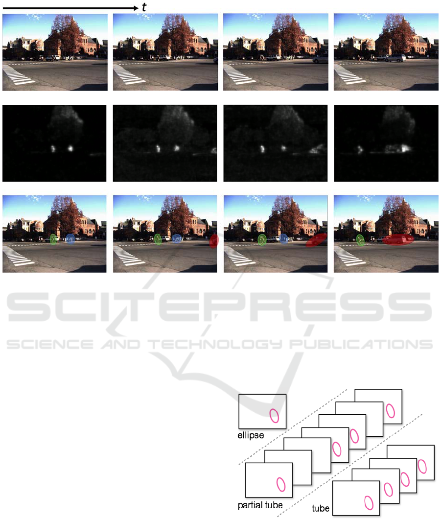
Figure 1: Subsequent frames of three separate processes. The first row is the input video. The second row is a simulated output
of the magnocellular pathway in the human visual system. We use it to extract low frequency motion information. Bright
pixels correspond to detected motion, while dark pixels correspond to a lack thereof. The third row is the result of our method.
Note that ellipses are constructed around groups of moving pixels.
localization techniques, temporal or spatiotemporal,
use CNNs to analyze video to make a single
determination about how the action of interest should
be isolated (Simonyan and Zisserman, 2014; Gkioxari
and Malik, 2015; Tran et al., 2015; Caelles et al.,
2016; Shou et al., 2016; Zhang et al., 2016). In a
departure from previous work, we propose a method
to handle simultaneous action localization of multiple
targets. As a result, performing our method on
available datasets and benchmarks limits the potential
questions.
3 OVERVIEW OF APPROACH
The primary goal is to spatially and temporally
localize each separate moving foreground entity in
videos “from the wild.” Furthermore, we suggest a
localization tool that also functions as a compact
representation of each entity’s motion. We
accomplish this by enclosing each moving
foreground entity within a tube, a sequence of ellipses
on consecutive frames as illustrated in Figure 2. Each
ellipse exists on a single frame and encloses a
temporal cross section of a moving entity. Each
ellipse is represented by an eight-element vector of
ellipse properties. For an ellipse e, the ellipse vector
is
e = [x, y, a, b, ϕ, f, Vx, Vy], (1)
Figure 2: A visualization of an ellipse, a partial tube, and a
tube. Note that the ellipse exists on a single frame and its
descriptor contains the center location, size, rotation angle,
frame present, and velocity. Both the partial tube and tube
are lists of ellipses. A partial tube does not contain ellipses
at dense frames. A tube does.
Feedforward and Feedback Processing of Spatiotemporal Tubes for Efficient Object Localization
379
where (x, y) is the center of the ellipse and a, b, and ϕ
are the semi-major axis length, semi-minor axis
length, and the angle of rotation (counterclockwise
from the x-axis to the major axis) respectively.
Property f is the frame of the video where the ellipse
is present and Vx and Vy are the Cartesian velocity
components of this ellipse at frame f. The x property
of ellipse e is denoted e
x
.
We detail and propose a four-step process to
create tubes from input video data. Given a video with
T frames {F
t
}
t=1…T
we find a list of tubes such that
each encompasses a foreground object. Note that
none of the following methods require the use of
spatial information.
3.1 Alg. 1: Magnocellular Motion
Processing
At each video frame, we invoke the work of (Benoit
et al., 2010) to perform biologically inspired low
level image processing replicating the magnocellular
retino-thalamic pathway of the mammalian visual
system. This method is distinct from typical
“background subtraction” schemes due to the
presence of a relative sensitivity and memory/time
decay associated with identified motion. This
naturally introduces a hierarchical attention span
based on relative size, magnitude of motion, and
motion duration.
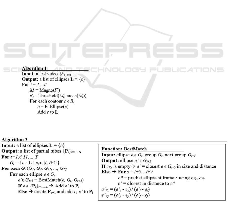
Algorithm 1 reads the input video and creates a
list of ellipses that spatially enclose foreground
moving objects.
Notably, the output of this magnocellular
processing provides motion information that would
be completely unavailable from individual still
frames alone. The method captures motion that is
abstracted from average motion spanning multiple
frames. The identified pixel locations are reduced via
a threshold set according to the mean pixel value in
the magnocellular output. This creates a binary image
with groups of “activated” pixels, which we erode
then dilate.
An ellipse is then fitted around each surviving
group of pixels. After filtering out ellipses with a
semi-major axis less than equal to five pixels, each
ellipse’s identifying information is stored onto a list.
The result is a list of ellipses, each of which enclose a
moving object in the foreground.
3.2 Alg. 2: Constructing Partial Tubes
The list of ellipses becomes input to the creation of a
sequence of ellipses, termed a partial tube. This is our
primary attempt at locating an entity across time.
First, the ellipses are gathered in groups G
t
based on
the frame number, f, of each. Since only one ellipse is
selected per partial tube per group, the width of the
bin (in frames) is a hyperparameter. A larger bin size
encourages a scarcer localization of the entity across
time. In the limit as bin size is decreased, Algorithm
2 approaches a frame-by-frame analysis. We chose
our bin size as 5 frames (i.e., ellipses in frame 6-10
are in a group, ellipses in 11-15 are in the next group,
etc.). We then pair each ellipse in a group with its
“best match” in the next group.
Algorithm 2 organizes the list into paths that
represent an entity’s motion through time.
The best match is defined as follows. Let ellipse e
ϵ G
t
and ellipse g ϵ G
t+5
. If velocity information is
available for e, we use it to create a “prediction
ellipse” at the expected location of e in each frame in
G
t+5
. Then, g is the best match ellipse if and only if it
is
the
closest
of
all
ellipses in G
t+5
to its prediction
ICPRAM 2019 - 8th International Conference on Pattern Recognition Applications and Methods
380
ellipse. If the velocity information does not yet exist
(i.e., the ellipse belongs to the first group in the video
or is the start of a new entity), g is the best match to e
if and only if it is the closest in G
t+5
to e via size and
distance.
Once an ellipse pairing occurs, two important
things happen. First, since we assume the pair of
ellipses are two different temporal cross sections of
the same object, we can calculate the velocity (in
pixels/frame) between the center of each ellipse using
the forward difference method. This information is
stored simply as two scalar properties, Vx and Vy, of
the latter ellipse. Second, pairs of ellipses are stored
as partial tubes unless the former ellipse of the pair
already belongs to another partial tube. In that case,
the latter ellipse in the pair is simply appended to the
same partial tube.
We iterate through the frames of the video
repeating the grouping and pairing process, to create
partial tubes. Each partial tube is a list of ellipses that
corresponds to one potential foreground object.
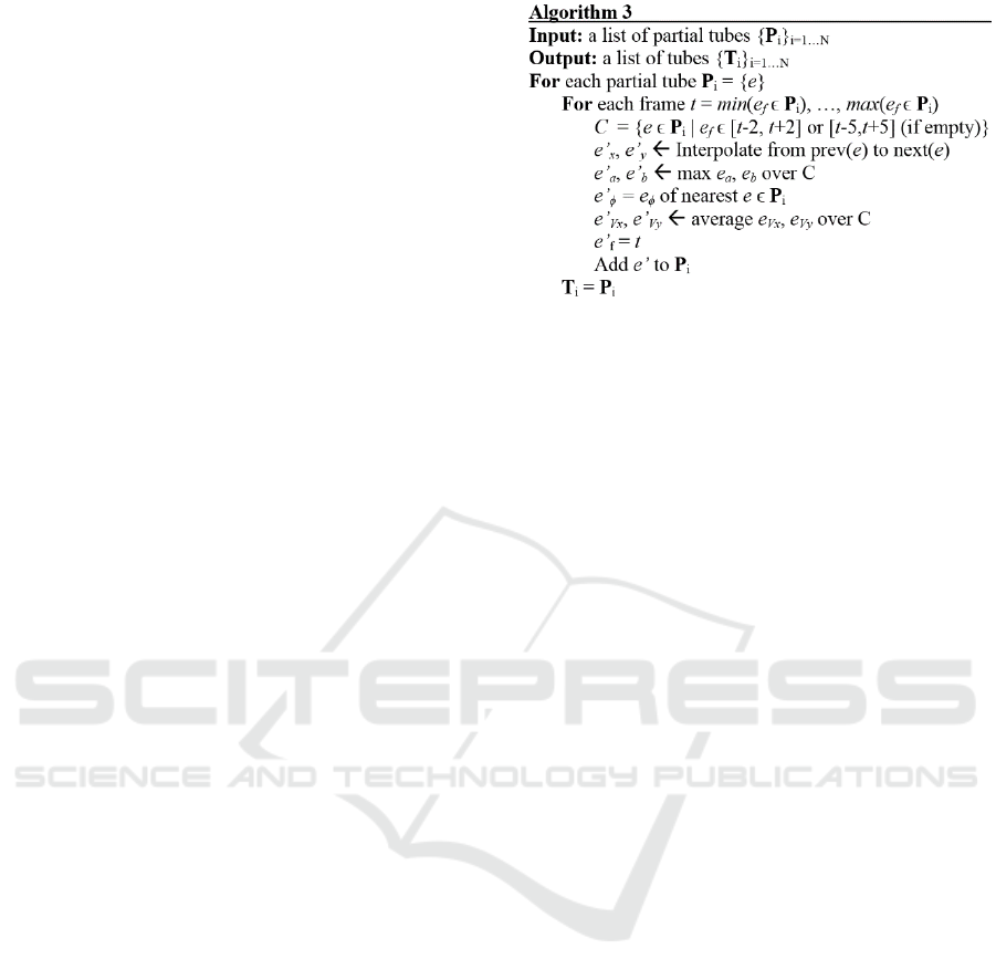
3.3 Alg. 3: Tube Completion
The partial tubes create a sparse localization of the
potential foreground entities in the video, existing
approximately once per every bin size, unlike the
continuously present entities they are meant to
represent. For the representation to be like the entity,
an ellipse must exist at every frame between the start
and end frames of the entity. Algorithm 3 makes tubes
by defining and creating ellipses between existing
ellipses in the partial tube.
We consider each partial tube separately. For
every frame, t, in a partial tube, P, we construct a
group, C, that consists of every ellipse e ϵ P “near”
frame t. To be near frame t is to be within half of
binsize (rounded down to nearest integer) away from
t (i.e., e
f
ϵ [t-2, t+2]). If nothing is near t, we extend
the definition to include any ellipse within binsize of
t (i.e., e
f
ϵ [t-5, t+5]). The ellipses grouped in C are
used to artificially smooth the properties of the ellipse
at t.
At each frame, we check if an ellipse exists in the
partial tube. If it does, the ellipse becomes a part of
the new tube. Otherwise, we interpolate the value of
the new x and y coordinates using the nearest ellipses
before and after frame t. The a and b properties of our
new ellipse are defined as the maximum a and b
values across C. The orientation, ϕ, of the new ellipse
is chosen as the ϕ of the closest ellipse in the partial
tube. The velocities, Vx and Vy, are defined as the
average Vx and Vy across C.
Algorithm 3 interpolates between sparse ellipses
in each partial tube to create a tube, the union of a
sequence of ellipses across consecutive frames.
After repeating the grouping and interpolating
process for each frame in the partial tube, the result is
a list of ellipses at every frame. This representation,
shown in Figure 3, is henceforth referred to as a tube.
The process is repeated for each partial tube, resulting
in a list of tubes.
3.4 Alg. 4: Tube Merging
Immediately after tube creation, a single entity, as
defined by human perception, is occasionally
represented by a union of several tubes instead of a
single tube. Usually, this is a result of one or more
occlusions. Consider the case shown in Figure 3. In
the first video, the pedestrian on the left is represented
by two separate tubes. By connecting those tubes
across the occlusion, we keep track of the entity.
Algorithm 4 connects tubes that likely cover the same
entity. To that end, we must first define a prediction
horizon, k, a positive integer denoting the number of
frames to look before/after a tube to determine its
potential connection. We consider each tube
separately. When considering a tube, we check for
other tubes that begin k frames after the end of (or that
end k frames before the start of) the tube.
Consider finding a second tube to connect to tube
T. First, we calculate an average Vx and Vy across the
first (and last) frames of T. Using this velocity vector,
we create a prediction ellipse where the entity would
be k frames before the beginning and after the end of
T. The prediction ellipse is compared with the
beginning and end of the other tubes. We determine
the tube that either begins (if the prediction ellipse is
after T) or ends (if the prediction ellipse is before T)
closest in space to the prediction ellipse and call this
potential match U. If the prediction ellipse is within a
spatial threshold (we chose 100 pixels) of U at the
same
frame and both tubes have similar velocity
Feedforward and Feedback Processing of Spatiotemporal Tubes for Efficient Object Localization
381
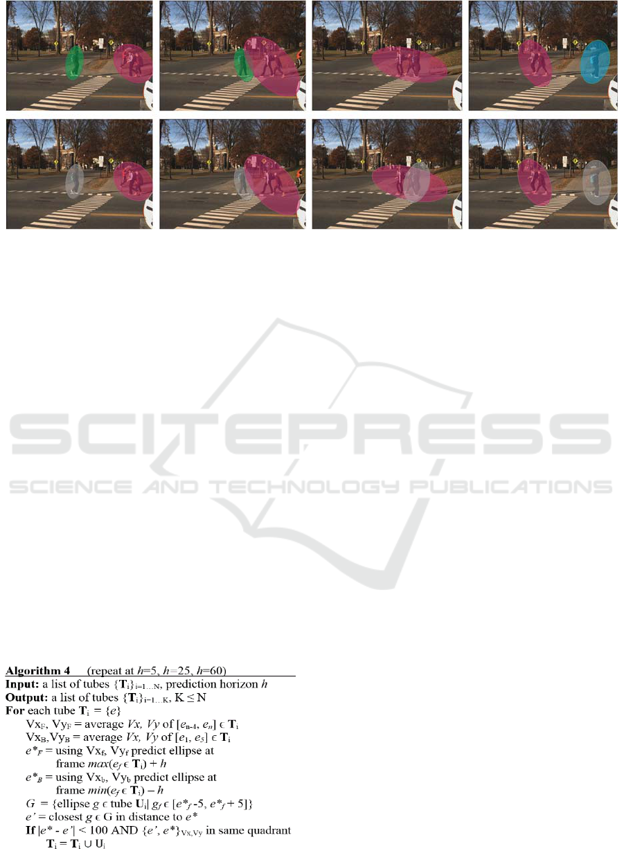
Figure 3: A scene before (top) and after (bottom) the implementation of Algorithm 4. The pedestrian with the backpack is
occluded by the group of people walking oppositely. In the first video, the pedestrian’s tube ends at the occlusion and a new
tube begins once the group has passed. In the second video, we can keep track of the pedestrian even during the occlusion.
vectors (Vx and Vy signs match unless |V| <1), we
combine the tubes into one. Otherwise, T remains
unmatched. When two tubes are combined, the
properties of the ellipses between the two tubes are
interpolated.
We repeat this tube connecting process for all
tubes. Furthermore, we conduct the process thrice,
each at a different value of k (k = 5, k = 25, and k =
60). This connects tubes across occlusions up to two
seconds long.
4 TOP DOWN STRATEGIES
Our localization framework offers the opportunity to
insert feedback loops that use preliminary results to
improve the quality of the tubes. We believe this is an
advantage for scalability. In this section, we detail
some of our feedback loops, which we denote as top-
down methods. The methods discussed are not an
exhaustive list, as we believe the possibilities for top
down solutions are numerous.
Algorithm 4 connects tubes separated by several
frames.
4.1 Magnocellular Sensitivity
As previously stated, the magnocellular-inspired low
level image processing uses relative sensitivity to
introduce an attention span based on size and motion.
When a large, quickly moving object exits the frame,
it creates a change in sensitivity. This effect increases
the intensity value of the pixels in the magnocellular
output as shown in Figure 4.
A false match created by a sensitivity effect is
detrimental to the system’s ability to keep track of an
object. Rigid pairwise matching schemes experience
difficulty with such outlier frames. Our sparse
matching approach in Algorithm 2 is more robust to
outlier frames.
In long periods with relatively small amounts of
motion, the sensitivity effect can last for consecutive
frames. To prevent the system from creating false
matches as a result, we incorporate our knowledge
about the tubes before and after the sensitivity effect.
We measure pixel intensities in each frame of the
magnocellular output to detect the temporal borders
of the prolonged sensitivity effect. Empirically, we
expect a majority of pixels to be dark or mostly dark
(intensity = 0–5). When the total number of non-dark
pixels surpass the total number of dark pixels in a
frame, we consider the frame a product of
oversensitivity. Intermittent spikes of sensitivity are
usually manageable because of our implementation of
Algorithm 2, while prolonged areas of sensitivity can
indicate a need for top-down solutions.
ICPRAM 2019 - 8th International Conference on Pattern Recognition Applications and Methods
382
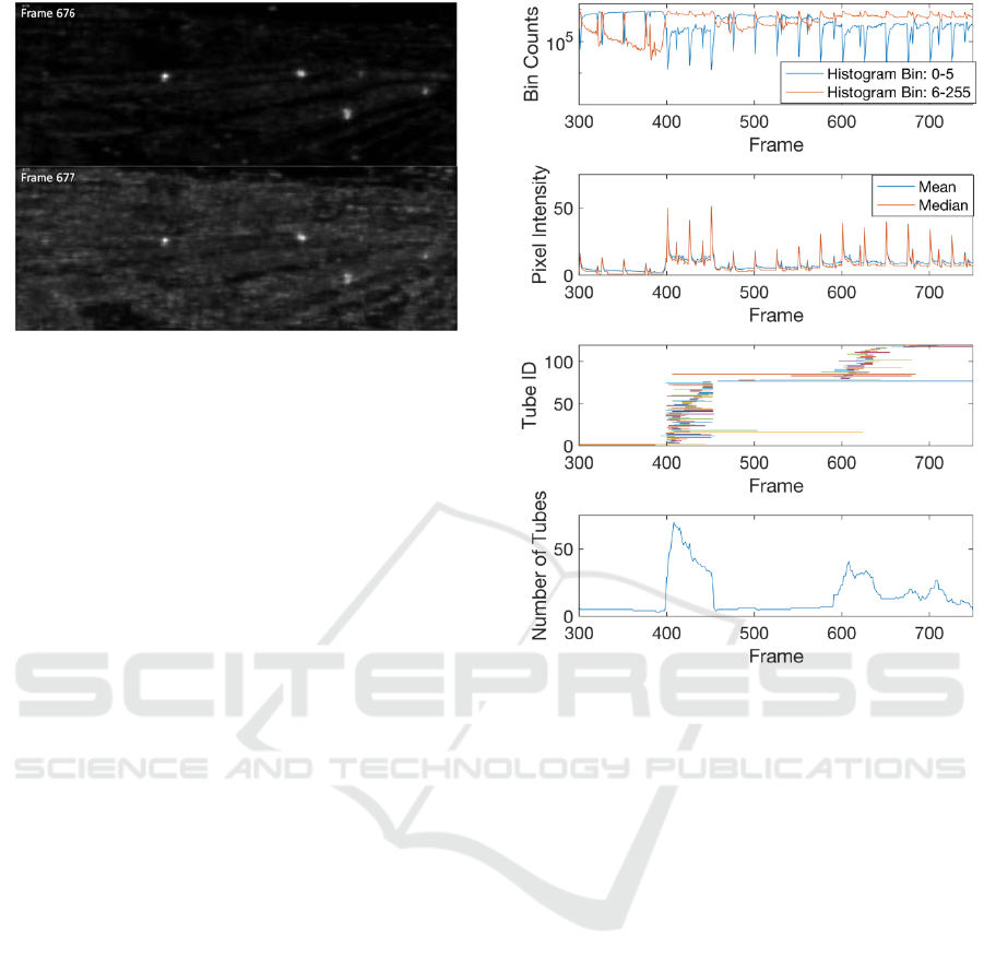
Figure 4: The visual result of a spike in magnocellular
sensitivity. Analysis of this effect tells us when to consider
top-down strategies.
We believe cases of prolonged sensitivity are
regions that require feedback paths to repair
trajectories in the region. In addition to measuring
pixel intensities, we can also use our preliminary tube
results to detect magnocellular sensitivity. For
example, we consider the number of tubes present in
each frame. The magnocellular sensitivity creates a
large number of tubes that are short in duration. The
sudden increase in the number of tubes corresponds
to the area of sensitivity, as shown in Figure 5.
Recognizing this phenomenon via the tube
information from the first pass demonstrates our
approach’s unique propensity for incorporating
feedback loops.
To remedy the effect of magnocellular sensitivity,
we consider the tubes present immediately before and
after the sensitivity effect. Using the velocity
information from the former tube, we predict where
we expect it to be after the effect. If a tube begins after
the effect within a location threshold (we chose 100
pixels), we connect the tubes and interpolate the
ellipse values between them.
4.2 Segmenting Object Tracks
An existing tube trajectory may need to be segmented
for either of two reasons. The first is that the
trajectory is corrupted with noise, in which case the
spurious trajectory may be flagged. The second is that
a tube trajectory may change to a different object;
sometimes, multiple objects are caught in one tube
track. Reasons for this may be that two objects
became close to each other and were merged, or after
one object stopped, a nearby object had similar
motion characteristics and the initial tube
construction therefore combined them. An example
of this is shown in Figure 6. We can clearly see in a
Figure 5: Histogram intensity counts of a magnocellular
output (top). We consider magnocellular sensitivity when
the orange line is above its blue counterpart. These same
patterns are emulated in the mean and median pixel
intensity lines (second). Tube identities and durations
(third) are shown along with the number of tubes in each
frame (last). Either of the above can be used to detect
magnocellular sensitivity.
qualitative manner how the trajectory shifts from one
object to another; fortunately, we can clearly see the
difference in the trajectories as well.
The correct subset of trajectories clusters well in
space and time. Algorithm 5 identifies these clearly
different trajectories and re-labels them as separate
tubes. Algorithm 5 is a feedback process that does not
necessarily have to be performed on every tube.
Algorithm 5 segments a given tube into smaller
sections of consistent trajectories. After
segmentation, the algorithm also recombines the
sections. In this manner, noisy areas of the trajectory,
or areas where the trajectory clearly shifted to another
object are identified as separate tubes.
Feedforward and Feedback Processing of Spatiotemporal Tubes for Efficient Object Localization
383
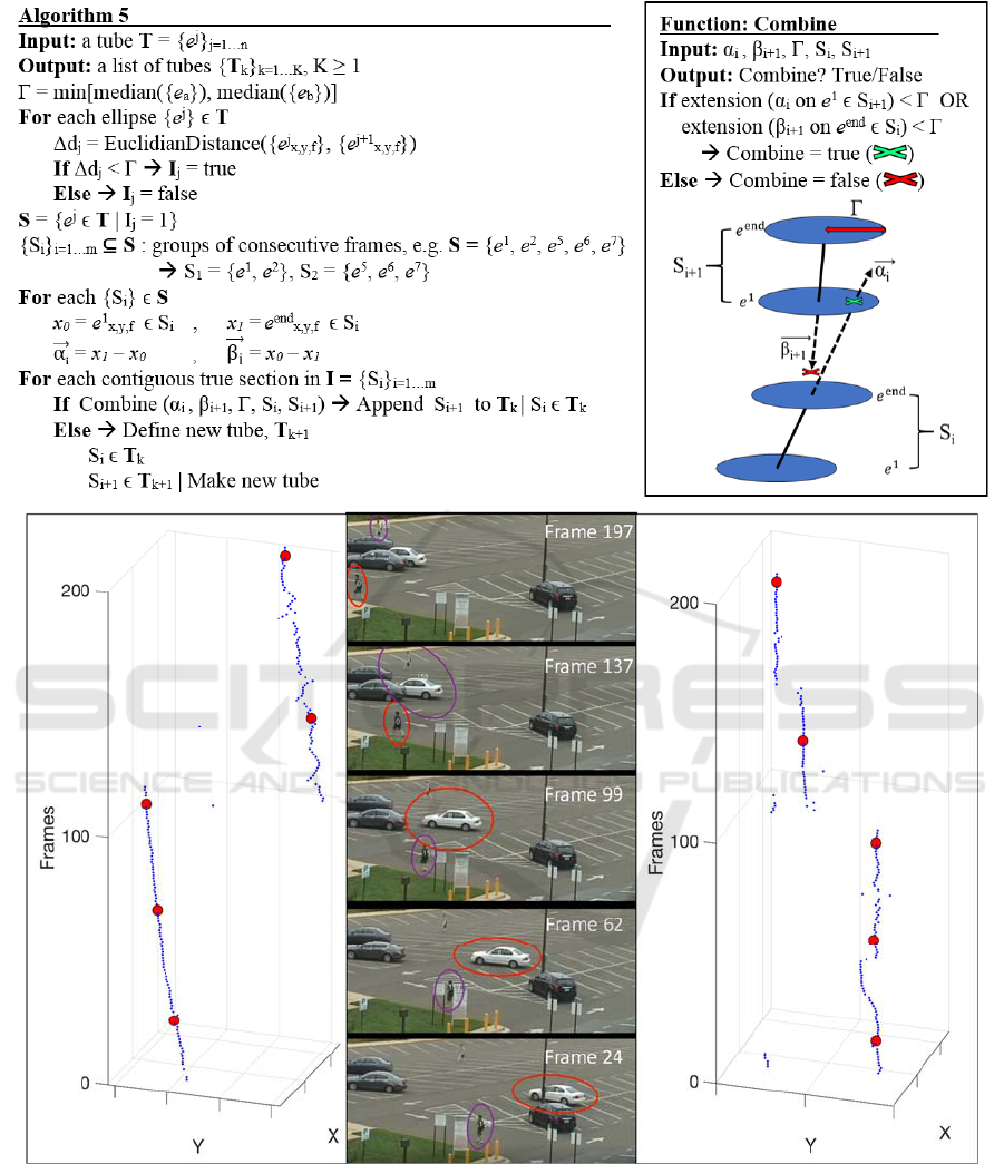
Figure 6: In the center, we see an example of tubes switching objects as they track. The red tube (left) follows the car as it
moves across the parking lot, and then switches to the nearby pedestrian. Meanwhile, the purple tube (right) began on the
pedestrian track and switched to the car, and then to another pedestrian. The dots in either trajectory correspond to the frames
shown in the video (center).
ICPRAM 2019 - 8th International Conference on Pattern Recognition Applications and Methods
384
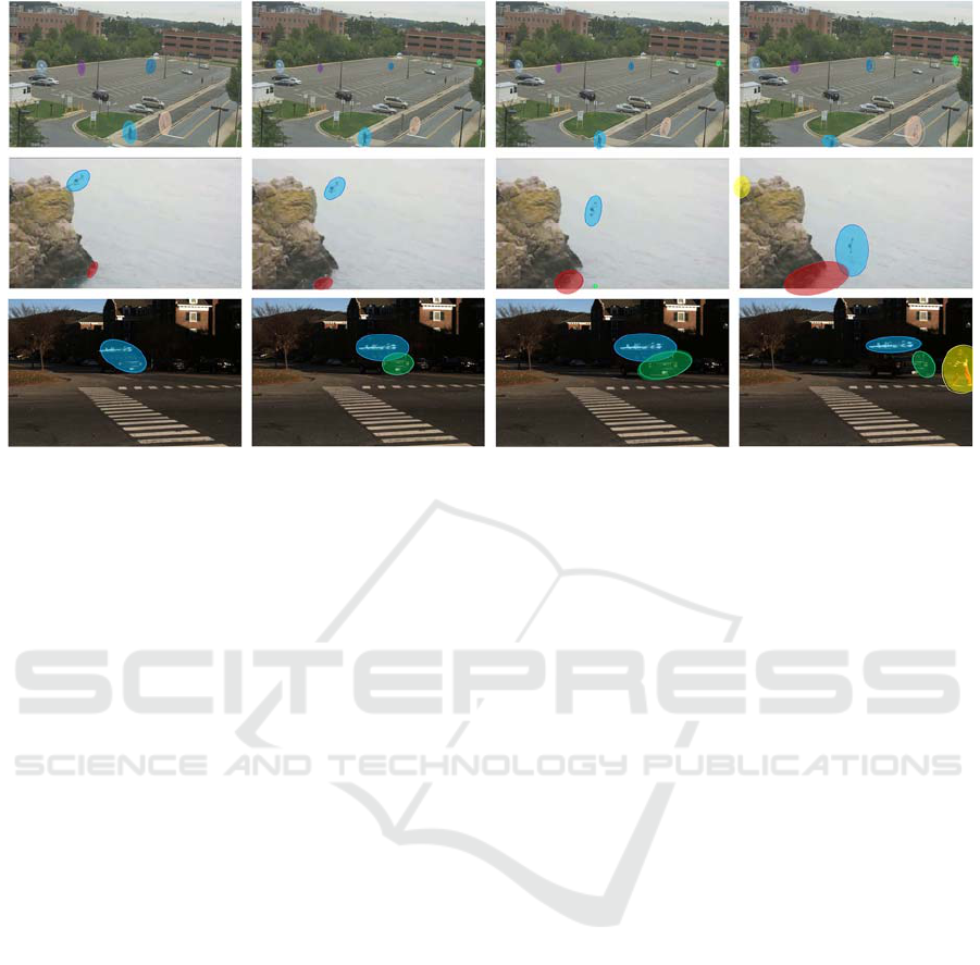
Figure 7: Three videos from separate datasets illustrating the results of our method. (Top) row is from the VIRAT video
dataset, (middle) is from Thumos-15, and (bottom) is from our recorded dataset (Oh et al., 2011; Gorban et al., 2015; Ray
and Miao, 2016) .
5 CONCLUSIONS
Action localization methods often require training
data, supervision, and/or dense motion information.
In this paper, we have presented a novel approach that
performs unsupervised spatiotemporal action
localization on videos in the wild without any of this
information.
Our framework simultaneously localizes multiple
actions and creates a compact macro representation of
the associated spatiotemporal motion for each.
Additionally, our approach does not require spatial
information. Subsequent incorporation of spatial
information within this framework offers exciting
opportunity for improvement. For the above reasons,
we believe our approach provides a strong foundation
for object/action classification as well as broad
possibility for top-down improvements.
ACKNOWLEDGEMENTS
We are grateful to Chris Kymn who contributed
valuable ideas and approaches to this work. This
work is supported in part by grants from the Office of
Naval Research award number N00014-16-1-2359.
REFERENCES
Benoit, A., Caplier, A., Durette, B., & Hérault, J. (2010).
Using human visual system modeling for bio-inspired
low level image processing. Computer vision and
Image understanding, 114(7), 758-773.
Brox, T., & Malik, J. (2011). Large displacement optical
flow: descriptor matching in variational motion
estimation. IEEE transactions on pattern analysis and
machine intelligence, 33(3), 500-513.
Brox, T., & Malik, J. (2010, September). Object
segmentation by long term analysis of point
trajectories. In European conference on computer
vision (pp. 282-295). Springer, Berlin, Heidelberg.
Caelles, S., Maninis, K. K., Pont-Tuset, J., Leal-Taixé, L.,
Cremers, D., & Van Gool, L. (2017). One-shot video
object segmentation. In CVPR 2017. IEEE.
Chang, J., Wei, D., & Fisher, J. W. (2013). A video
representation using temporal superpixels. In
Proceedings of the IEEE Conference on Computer
Vision and Pattern Recognition (pp. 2051-2058).
Fulkerson, B., Vedaldi, A., & Soatto, S. (2009, September).
Class segmentation and object localization with
superpixel neighborhoods. In Computer Vision, 2009
IEEE 12th International Conference on (pp. 670-677).
IEEE.
Galasso, F., Shankar Nagaraja, N., Jimenez Cardenas, T.,
Brox, T., & Schiele, B. (2013). A unified video
segmentation benchmark: Annotation, metrics and
analysis. In Proceedings of the IEEE International
Conference on Computer Vision (pp. 3527-3534).
Gavrila, D. M. (1999). The visual analysis of human
movement: A survey. Computer vision and image
understanding, 73(1), 82-98.
Feedforward and Feedback Processing of Spatiotemporal Tubes for Efficient Object Localization
385

Giese, M. A., & Poggio, T. (2003). Cognitive neuroscience:
neural mechanisms for the recognition of biological
movements. Nature Reviews Neuroscience, 4(3), 179.
Gkioxari, G., & Malik, J. (2015). Finding action tubes.
In Proceedings of the IEEE conference on computer
vision and pattern recognition (pp. 759-768).
Gorban, A., Idrees, H., Jiang, Y. G., Zamir, A. R., Laptev,
I., Shah, M., & Sukthankar, R. (2015). THUMOS
challenge: Action recognition with a large number of
classes.
Grundmann, M., Kwatra, V., Han, M., & Essa, I. (2010,
June). Efficient hierarchical graph-based video
segmentation. In Computer Vision and Pattern
Recognition (CVPR), 2010 IEEE Conference on (pp.
2141-2148). IEEE.
He, K., Zhang, X., Ren, S., & Sun, J. (2016). Deep residual
learning for image recognition. In Proceedings of the
IEEE conference on computer vision and pattern
recognition (pp. 770-778).
Horn, B. K., & Schunck, B. G. (1981). Determining optical
flow. Artificial intelligence, 17(1-3), 185-203.
Jain, M., Van Gemert, J., Jégou, H., Bouthemy, P., &
Snoek, C. G. (2014). Action localization with tubelets
from motion. In Proceedings of the IEEE conference on
computer vision and pattern recognition (pp. 740-747).
Jain, S. D., & Grauman, K. (2014, September). Supervoxel-
consistent foreground propagation in video.
In European Conference on Computer Vision (pp. 656-
671). Springer, Cham.
Jiang, Y. G., Liu, J., Zamir, A. R., Toderici, G., Laptev, I.,
Shah, M., & Sukthankar, R. (2014). THUMOS
challenge: Action recognition with a large number of
classes.
Krizhevsky, A., Sutskever, I., & Hinton, G. E. (2012).
Imagenet classification with deep convolutional neural
networks. In Advances in neural information
processing systems (pp. 1097-1105).
Kuehne, H., Jhuang, H., Stiefelhagen, R., & Serre, T.
(2013). Hmdb51: A large video database for human
motion recognition. In High Performance Computing in
Science and Engineering ‘12 (pp. 571-582). Springer,
Berlin, Heidelberg.
Lee, Y. J., Kim, J., & Grauman, K. (2011, November). Key-
segments for video object segmentation. In Computer
Vision (ICCV), 2011 IEEE International Conference
on (pp. 1995-2002). IEEE.
Lu, Z. L., & Sperling, G. (1995). The functional
architecture of human visual motion perception. Vision
research, 35(19), 2697-2722.
Narayana, M., Hanson, A., & Learned-Miller, E. (2013).
Coherent motion segmentation in moving camera
videos using optical flow orientations. In Proceedings
of the IEEE International Conference on Computer
Vision (pp. 1577-1584).
Nguyen, A., Yosinski, J., & Clune, J. (2015). Deep neural
networks are easily fooled: High confidence predictions
for unrecognizable images. In Proceedings of the IEEE
Conference on Computer Vision and Pattern
Recognition (pp. 427-436).
Oh, S., Hoogs, A., Perera, A., Cuntoor, N., Chen, C. C.,
Lee, J. T., ... & Swears, E. (2011, June). A large-scale
benchmark dataset for event recognition in surveillance
video. In Computer vision and pattern recognition
(CVPR), 2011 IEEE conference on (pp. 3153-3160).
IEEE.
Oram, M. W., & Perrett, D. I. (1996). Integration of form
and motion in the anterior superior temporal
polysensory area (STPa) of the macaque
monkey. Journal of neurophysiology, 76(1), 109-129.
Pathak, D., Girshick, R. B., Dollár, P., Darrell, T., &
Hariharan, B. (2017, July). Learning Features by
Watching Objects Move. In CVPR (Vol. 1, No. 2, p. 7).
Perazzi, F., Pont-Tuset, J., McWilliams, B., Van Gool, L.,
Gross, M., & Sorkine-Hornung, A. (2016). A
benchmark dataset and evaluation methodology for
video object segmentation. In Proceedings of the IEEE
Conference on Computer Vision and Pattern
Recognition (pp. 724-732).
Polana, R., & Nelson, R. (1994, November). Low level
recognition of human motion (or how to get your man
without finding his body parts). In Motion of Non-
Rigid and Articulated Objects, 1994., Proceedings of
the 1994 IEEE Workshop on(pp. 77-82). IEEE.
Poppe, R. (2010). A survey on vision-based human action
recognition. Image and vision computing, 28(6), 976-
990.
Ray, L., & Miao, T. (2016, June). Towards Real-Time
Detection, Tracking and Classification of Natural
Video. In Computer and Robot Vision (CRV), 2016
13th Conference on(pp. 236-241). IEEE.
Roth, S., Lempitsky, V., & Rother, C. (2009). Discrete-
continuous optimization for optical flow estimation.
In Statistical and Geometrical Approaches to Visual
Motion Analysis (pp. 1-22). Springer, Berlin,
Heidelberg.
Shi, J., & Malik, J. (2000). Normalized cuts and image
segmentation. IEEE Transactions on pattern analysis
and machine intelligence, 22(8), 888-905.
Shou, Z., Wang, D., & Chang, S. F. (2016). Temporal
action localization in untrimmed videos via multi-stage
cnns. In Proceedings of the IEEE Conference on
Computer Vision and Pattern Recognition (pp. 1049-
1058).
Simonyan, K., & Zisserman, A. (2014). Two-stream
convolutional networks for action recognition in
videos. In Advances in neural information processing
systems (pp. 568-576).
Soomro, K., Zamir, A. R., & Shah, M. (2012). UCF101: A
dataset of 101 human actions classes from videos in the
wild. arXiv preprint arXiv:1212.0402.
Tokmakov, P., Schmid, C., & Alahari, K. (2017). Learning
to Segment Moving Objects. arXiv preprint
arXiv:1712.01127.
Tran, D., Bourdev, L., Fergus, R., Torresani, L., & Paluri,
M. (2015). Learning spatiotemporal features with 3d
convolutional networks. In Proceedings of the IEEE
international conference on computer vision (pp. 4489-
4497).
ICPRAM 2019 - 8th International Conference on Pattern Recognition Applications and Methods
386

Tsai, D., Flagg, M., Nakazawa, A., & Rehg, J. M. (2012).
Motion coherent tracking using multi-label MRF
optimization. International journal of computer vision,
100(2), 190-202.
Tsai, Y. H., Yang, M. H., & Black, M. J. (2016). Video
segmentation via object flow. In Proceedings of the
IEEE Conference on Computer Vision and Pattern
Recognition (pp. 3899-3908).
Wang, H., Kläser, A., Schmid, C., & Liu, C. L. (2011,
June). Action recognition by dense trajectories. In
Computer Vision and Pattern Recognition (CVPR),
2011 IEEE Conference on (pp. 3169-3176). IEEE.
Zhang, B., Wang, L., Wang, Z., Qiao, Y., & Wang, H.
(2016). Real-time action recognition with enhanced
motion vector CNNs. In Proceedings of the IEEE
Conference on Computer Vision and Pattern
Recognition (pp. 2718-2726).
Feedforward and Feedback Processing of Spatiotemporal Tubes for Efficient Object Localization
387
