
Unsupervised Fine-tuning of Optical Flow for Better Motion Boundary
Estimation
Taha Alhersh and Heiner Stuckenschmidt
Data and Web Science Group, University of Mannheim, 68131 Mannheim, Germany
Keywords:
Optical Flow, Unsupervised Learning, Fine-tuning, Motion Boundary, Deep Learning.
Abstract:
Recently, convolutional neural network (CNN) based approaches have proven to be successful in optical flow
estimation in the supervised as well as in the unsupervised training paradigms. Supervised training requires
large amounts of training data with task specific motion statistics. Usually, synthetic datasets are used for this
purpose. Fully unsupervised approaches are usually harder to train and show weaker performance, although
they have access to the true data statistics during training. In this paper we exploit a well-performing pre-
trained model and fine-tune it in an unsupervised way using classical optical flow training objectives to learn
the dataset specific statistics. Thus, per dataset training time can be reduced from days to less than 1 minute.
Specifically, motion boundaries estimated by gradients in the optical flow field can be greatly improved using
the proposed unsupervised fine-tuning.
1 INTRODUCTION
Despite the advances in computation, optical flow es-
timation is still an open and active research area in
computer vision. Optical flow can be considered as
a variational optimization problem to find pixel cor-
respondences between any two consecutive frames
(Horn and Schunck, 1981). Research paradigms in
this field have evolved from considering optical flow
estimation as a classical problem (Brox and Malik,
2011), to more high-level approaches using machine
learning, for example, convolutional neural networks
(CNN) as state-of-the-art method (Dosovitskiy et al.,
2015; Ilg et al., 2017; Wannenwetsch et al., 2017; Sun
et al., 2018).
Training convolutional neural networks (CNN)
to predict generic optical flow requires a massive
amount of training data, big computational power e.g.
Graphics Processing Units (GPU). However, obtain-
ing ground truth for realistic videos which is very
hard to achieve (Butler et al., 2012), and simply not
available in some scenarios. To overcome this prob-
lem, unsupervised learning frameworks have been
proposed. In such way, we can utilize the resources of
unlabeled videos (Jason et al., 2016). The idea behind
unsupervised methods is not to include ground truth
optical flow in training convolutional neural network,
nevertheless, using a photometric loss that measures
the difference between the target image and the (in-
verse / forward) warped subsequent image based on
a generated dense optical flow field predicted from
the convolutional networks. Hence, an end-to-end
convolutional neural network can be trained with any
amount of unlabeled image pairs, which helps in over-
coming the need of ground truth optical flow as train-
ing input.
Researchers have generated many pre-trained op-
tical flow estimation models either in supervised or
unsupervised way. The amount of effort and train-
ing time to produce such models is big. However,
fine-tuning on existing pre-trained models for spe-
cific purpose datasets will help in reducing effort and
time. The purpose of this paper is not to compete with
supervised state-of-the-art approaches, where ground
truth training data is available. In contrast, we aim
to provide a method that facilitates fast fine-tuning of
optical flow networks in scenarios where little to no
training data is available. Thus, we are proposing an
unsupervised fine-tuning approach for optical flow es-
timation with four main contributions: First, we intro-
duce an unsupervised loss function based on classical,
variational optical flow methods. Fine-tuning in an
unsupervised way might address the lack of of ground
truths. Also, it will work as catalyst for special pur-
pose datasets specially in real life scenarios. Second,
we reduce the time of training a CNN from scratch
- needs couple of days - and benefit from the pre-
trained models during fine-tuning which needs less
776
Alhersh, T. and Stuckenschmidt, H.
Unsupervised Fine-tuning of Optical Flow for Better Motion Boundary Estimation.
DOI: 10.5220/0007343707760783
In Proceedings of the 14th International Joint Conference on Computer Vision, Imaging and Computer Graphics Theory and Applications (VISIGRAPP 2019), pages 776-783
ISBN: 978-989-758-354-4
Copyright
c
2019 by SCITEPRESS – Science and Technology Publications, Lda. All rights reserved

Figure 1: Qualitative results: Optical flow estimated on
KITTI 2012 upper part, and KITTI 2015 bottom part us-
ing our method FlowNet2-SD-unsup. Right bottom corner
shows optical flow color code used in this manuscript.
than 1 minute in our case. Our preliminary results
indicate that this new unsupervised loss model might
indeed be promising with regard to optical flow esti-
mation and time needed. Third, we provide analysis
of the effectiveness of classical optical flow optimiza-
tion objectives in the context of CNNs. Forth, object
appearances and statistics can be successfully learned
from only few unsupervised training examples, which
can be measured especially by our improvement in
motion boundary estimates.
2 RELATED WORK
Motivated by the success of CNNs in various com-
puter vision tasks, learning optical flow is gaining a
lot of attention nowadays. Learning process could
be divided into supervised and unsupervised learn-
ing. Supervised learning optical flow requires ground
truth. Most researchers are using synthetic datasets
(Dosovitskiy et al., 2015; Mayer et al., 2016) for
training their networks. For example, Dosovitskiy et
al. (Dosovitskiy et al., 2015) suggested two CNN net-
works: FlowNetSimple (FlowNetS) in which input
images are stacked both together and then fed them
through a generic network to decide how to process
the image pair to extract the motion information. The
second one is FlowNetCorr (FlowNetC) which in-
cludes a correlation layer that performs multiplicative
patch comparisons between two feature maps. Their
network succeeded in predicting optical flow at up to
10 image pairs per second.
By stacking several simple FlowNet models with
some modification to some and introduce a fusion
network, Ilg et al. (Ilg et al., 2017) achieved aston-
ishing results using FlowNet2. On the other hand, a
network smaller than FlowNet2 by 17 times PWC-
Net (Sun et al., 2018) was designed via pyramidal
processing, warping, and the use of a cost volume.
They adopted DenseNet architecture (Huang et al.,
2017), which directly connects each layer to every
other layer in a feed forward fashion. Their results
shows the advantage of combining deep learning with
domain knowledge, while obtaining competitive re-
sults compared to other methods. Ranjan and Black
(Ranjan and Black, 2017) introduced Spatial Pyramid
Network (SPyNet) combined classical coarse-to-fine
pyramid methods with deep learning for optical flow
estimation. SPyNet is 96% smaller and faster than
FlowNet, hence less memory is required which makes
it promising for embedded and mobile applications.
SPyNet learn to predict flow increment at each pyra-
mid level rather than minimizing a classical objective
function. LiteFlowNet has been developed by Hui et
al. (Hui et al., 2018) which is 30 times smaller in the
model size of FlowNet2 and 1.36 times faster in exe-
cution. They have drilled down the missed architec-
tural details in FlowNet2. They have introduced an ef-
fective flow inference at each pyramid level through a
lightweight cascaded network to improve optical flow
estimation accuracy and permits seamless incorpora-
tion of descriptor matching in the network. Moreover,
a flow regularization layer has been developed to ame-
liorate the issue of outliers and vague flow boundaries
by using a feature-driven local convolution.
Another research paradigm for CNNs adopts un-
supervised learning approach. FlowNet was adopted
while equipped with unsupervised Charbonnier loss
function to minimize photometric consistency which
measures the difference between the first input im-
age and the (inverse) warped subsequent image based
on the predicted optical flow by the network (Jason
et al., 2016; Ren et al., 2017). Alletto and Rigazio
(Alletto and Rigazio, 2017) used energy based gen-
erative adversarial network (EbGAN) consists of two
fully convolutional auto-encoders where the generator
network is attached with the interpolation of the two
input frames and outputs network is a pixel-level en-
ergy map instead of functioning as a binary classifier
between true or false. Interpolating between frames
was used by Long et al. (Long et al., 2016) to train
CNNs for optical flow estimation. Zhu et al. (Zhu
et al., 2017) argue that using optical flow estimators
to generate proxy ground truth data for training CNNs
could help in learn to estimate motion between image
pairs as good as using true ground truth. In order to
handle occlusion Wang et al. (Wang et al., 2018) pro-
posed an end-to-end network consists of two copies
of FlowNetS with shared parameters, one to produce
forward optical flow while the other one generates
backward warping which is used for occlusion mask.
Loss function used includes occlusion predicted by
motion. To tackle large motion estimation they have
introduced histogram equalizer and occlusion map for
the warped frame. Makansi et al. (Makansi et al.,
2018) proposed an assessment network that can learn
to predict the error form a set of optical flow fields
Unsupervised Fine-tuning of Optical Flow for Better Motion Boundary Estimation
777
generated with various optical flow estimation tech-
niques. Then, the assessment network is used as a
proxy ground truth generator to train FlowNet. The
later work is most related to our work except that we
focus on the effectiveness of implementing classical
optical flow optimization objectives in CNNs archi-
tecture. Janai et al. (Janai et al., 2018) learned optical
flow and occlusions together via modeling a temporal
relationship for three frames window by estimating
past and future optical flow. They have used photo-
metric loss function and explicitly reason about oc-
clusions.
Many motion boundary estimation methods de-
pends on optical flow (Papazoglou and Ferrari, 2013;
Wang et al., 2013; Weinzaepfel et al., 2015; Ilg et al.,
2018). Philippe Weinzaepfel et al. (Weinzaepfel
et al., 2015) suggetsed a learning-based method for
motion boundary detection based on random forests
since motion boundaries in local patch tends to have
similar patterns, static appearance and temporal fea-
tures, color, optical flow, image warping and back-
ward flow errors. In their work, Li et al. proposed
an unsupervised learning approach for edge detection.
This method utilizes two types of information as in-
put: motion information in the form of noisy semi-
dense matches between frames, and image gradients
as the knowledge for edges. The performance of mo-
tion boundary estimation is limited by several issues
like the removal of weak image edges as well as label
noises.
We have adopted FlowNet2-SD architecture
which is implemented in Caffe deep learning frame-
work, and considered as subnet of Flownet2 (Ilg
et al., 2017). FlowNet2-SD is a modified version of
FlowNetS but more deeper to deal with small dis-
placements. FlowNet2-SD architecture is illustrated
in Figure 2. We have replaced the final and interme-
diate losses with unsupervised losses described in the
following section.
Figure 2: FlowNet2-SD architecture which takes two input
images and produces optical flow (repainted from (Ilg et al.,
2017)).
3 NETWORK ARCHITECTURE
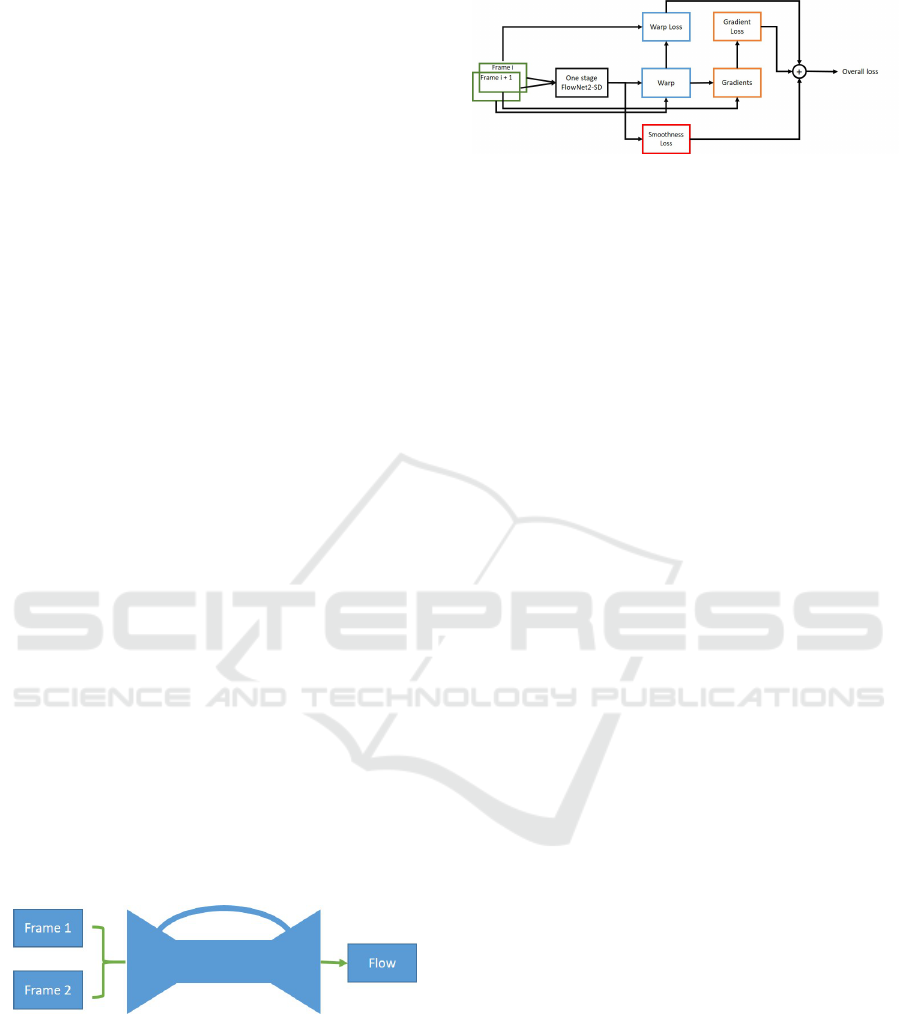
Figure 3 shows our proposed unsupervised loss. Only
one stage (resolution) is shown from multi-resolution
optical flow architecture adopted from FlowNet2-SD.
Figure 3: An overview of how unsupervised losses have
been constructed. Only one stage(resolution) of producing
flow from FlowNet2-SD is shown.
Stacking both input images together and feed them
to the network, allows the network to decide itself
how to process the image pair to extract the motion
information. In each stage (resolution) the loss is con-
structed using calculating three main losses:
• Warp loss: is calculated when second frame is
back warped with the produced optical flow and
calculate the difference between the generated
warped frame and frame one.
• Gradient loss: Calculate the difference between
gradients of warped image and gradients of frame
one.
• Smoothness loss: works as a penalizing term
through calculating the variation of generated
flow field in u and v directions.
3.1 Cost Functions
The cost function can be structured by combining
color, gradient and smoothness terms where I
1
,I
2
:
(Ω ⊂ R
2
) → R
3
are any two consecutive frames.
Also, x := (x, y)
T
are the point in Ω domain, and
w := (u, v)
T
is the optical flow field (Brox and Ma-
lik, 2011) as follows:
E(w) = E
color
+ γE
gradient
+ αE
smooth
(1)
Where the color energy E
color
is an assumption
that the corresponding points should have the same
color:
E
color
(w) =
Z
Ω
Ψ(|I
2
(x + w(x)) − I
1
(x)|
2
)dx (2)
The gradient energy E
gradient
is a constrain which
is invariant to additive brightness changes to deal with
the illumination effect:
E
gradient
(w) =
Z
Ω
Ψ(|∇I
2
+ w(x)) − ∇I
1
|
2
)dx (3)
Adding smoothness constrain E
smooth
works as
regularity term for penalizing the total variation of the
flow field generated from 2 and 3:
E
smooth
(w) =
Z
Ω
Ψ(|∇u(x)|
2
) − |∇v(x)|
2
)dx (4)
VISAPP 2019 - 14th International Conference on Computer Vision Theory and Applications
778
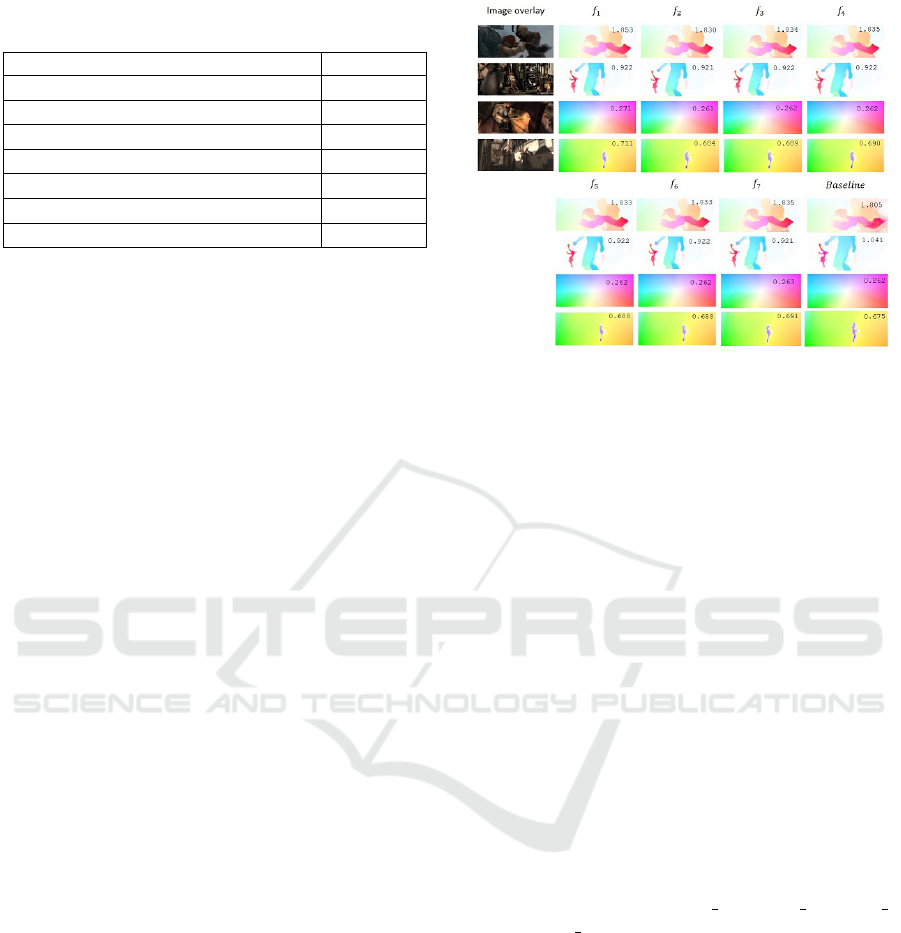
Table 1: Different combinations of cost function terms from
Equation 1 and their references used in this research.
Terms Reference
E
kcolork
2
+ γE
kgradientk
1
+ αE
ksmoothk
1
f
1
E
kcolork
2
+ γE
kgradientk
2
+ αE
ksmoothk
1
f
2
E
kcolork
1
+ γE
kgradientk
1
+ αE
ksmoothk
1
f
3
E
kcolork
2
+ αE
ksmoothk
1
f
4
E
kcolork
2
f
5
γE
kgradientk
1
+ αE
ksmoothk
1
f
6
γE
kgradientk
1
f
7
Ψ(s) represents different metrics as follow:
Ψ(s) =
ksk
1
,
s ∈ [E
color
(w),E
gradient
(w),E
smooth
(w)]
ksk
2
,
s ∈ [E
color
(w),E
gradient
(w),E
smooth
(w)]
(5)
Where,
ksk
1
=
n
∑
i=1
|y
i
− f (x
i
)| (6)
and
ksk
2
=
n
∑
i=1
(y
i
− f (x
i
))
2
(7)
Equation 5 shows the non-local functions used in our
approach. L
1
norm 6 and L
2
norm 7 were used for dif-
ferent combinations using color, gradient or smooth-
ness terms.
4 EXPERIMENTS
4.1 Datasets
Three well known datasets have been used for un-
supervised fine-tuning and testing predicted optical
flow:
4.1.1 KITTI 2012
(Geiger et al., 2012) is a real-world computer vision
benchmarks consists of 194 training image pairs and
195 image pairs for testing purposes.
4.1.2 KITTI 2015
(Menze and Geiger, 2015) is a benchmark containing
of 200 training scenes and 200 test scenes (4 color im-
ages per scene, saved in loss less png format). Com-
pared to KITTI 2012 benchmark, it covers dynamic
scenes for which ground truth was established in a
semi-automatic process.
Figure 4: Examples of optical flow estimated using different
combinations of cost functions based on Table 1 and EPE on
different Sintel validation sets. f
1−7
are the corresponding
cost function line in the mentioned table.
4.1.3 Sintel
(Butler et al., 2012) is an open source synthetic
dataset extracted from animated film produced by Ton
Roosendaal and the Blender Foundation. It contains
1041 image pairs for training and 552 image pairs
for testing both training and testing come with Clean
and Final versions. Those versions been used to in-
vestigate when optical flow algorithms break, so each
frame has been rendered in different pass: the Clean
pass, which contains shading, but no image degra-
dations, and the Final pass, which additionally in-
cludes motion blur, defocus blur, and atmospheric ef-
fects, and corresponds to the final movie (Wulff et al.,
2012).
Since Sintel training dataset provides optical flow
ground truth, which can be used for validating our ap-
proach, we have divided the training dataset into train-
ing (845 training image pairs) and validation (196
testing image pairs from alley 2, ambush 5, market 2
and sleeping 1 sequences) datasets for validating our
method.
Flying Chairs (Dosovitskiy et al., 2015) was not
used in this work since FlowNet2-SD model was
trained on it, and to avoid over fitting while fine-
tuning. Hence, we have decided not to include it.
4.2 Training Details
We have fine-tuned the pre-trained FlowNet2-SD
model (Ilg et al., 2017) in an unsupervised way and
called it FlowNet2-SD-unsup. Number of training
(fine-tuning) iteration was up to 50 iterations which
takes only 52 seconds on NVIDIA GeForce GTX
1080 Ti. Learning rate used was fixed to 1.0e
−7
.
Unsupervised Fine-tuning of Optical Flow for Better Motion Boundary Estimation
779
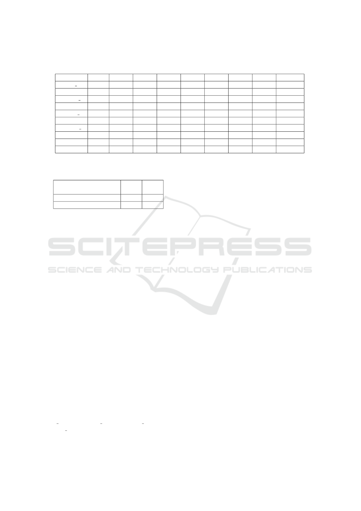
Table 2: EPE results for optical flow generated by our method FlowNet2-SD-ft-unsup using different loss function as described
in Table 1 and the FlowNet2-SD (Baseline) on various Sintel validation sequences.
f
1
f
2
f
3
f
4
f
5
f
6
f
7
Baseline
alley 2 Clean 0.520 0.517 0.521 0.531 0.521 0.520 0.520 0.518
Final 0.528 0.527 0.528 0.528 0.528 0.527 0.527 0.525
ambush 5 Clean 14.372 14.366 14.373 14.403 14.374 14.372 14.372 14.454
Final 15.612 15.612 15.613 15.612 15.612 15.611 15.611 15.625
market 2 Clean 0.936 0.935 0.936 0.940 0.937 0.937 0.937 0.941
Final 1.030 1.029 1.030 1.029 1.029 1.030 1.030 1.035
sleeping 1 Clean 0.237 0.235 0.238 0.246 0.237 0.237 0.237 0.234
Final 0.250 0.250 0.250 0.249 0.249 0.250 0.250 0.236
Average Clean 4.016 4.013 4.017 4.030 4.017 4.016 4.016 4.037
Final 4.355 4.355 4.355 4.354 4.354 4.355 4.354 4.355
Table 3: EPE results for evaluating our method on the vali-
dation sets of Sintel training with comparison to FlowNet2-
SD (Baseline).
Method Sintel Sintel
Clean Final
FlowNet2-SD (Baseline) 4.036 4.354
FlowNet2-SD-ft-unsup 4.016 4.354
5 RESULTS
5.1 Evaluation
We have reported optical flow quantitative evaluation
results with regard to average end point error (EPE)
for for Sintel validation sets in Table 3 while provided
only qualitative results for KITTI 2012, KITTI 2015
in Figure 1.
Quantitative results show that FlowNet-SD-unsup
achieved good results with comparison to baseline.
We are not in a situation to compete with fine-
tuning in supervised way (ground truth available) and
achieve better results, but to find a fast (in terms of
training and execution) and reasonable method to pro-
duce competitive optical flow when ground truth is
not given, i.e. real-world scenarios. Runtime for gen-
erating one optical flow file takes only 1.3e
−4
sec-
onds.
Evaluation for the validation dataset from Sintel
based on different combination of cost function de-
scribed in Table 1 fine-tuned on Sintel is shown in
Table 3.
Table 3 results show a small variation in the EPE
values for different settings. For example, using
L
2
norm for warping and gradient functions combined
with L
1
norm for smoothness achieved best results for
alley 2 clean, ambush 5 clean, market 2 clean and
sleeping 1 clean validation datasets. Baseline has
outperformed our approach in some final validation
sets with small margin. But, the average EPE for Fi-
nal validation sets form both FlowNet2-SD-unsup and
FlowNet2-SD is the same.
5.2 Motion Boundary Estimation
We have compared motion boundary estimation from
our method (FlowNet2-SD-unsup) and the baseline
(FlowNet2-SD). Our method outperform the baseline
by large margin in Sintel clean, while it was almost
the same for Sintel final, Table 4. There is an im-
provement also in quality of qualitative results which
is visible in Figure 5. The variation in motion in dif-
ferent validation sequences have produced different
F-measures in Table 4. One observation is that F-
measure score is correlated with number and magni-
tude of produced motion boundaries.
5.3 Qualitative Results
Visualizations of some generated examples of optical
flow are illustrated in Figure 4 for Sintel and in Fig-
ure 1 for KITTI 2012 and 2015. KITTI here represent
real world data, while Sintel exemplify synthetic sce-
nario. Our method succeeded in capturing fine struc-
ture results around edges, while FlowNet2-SD shows
smooth results as shown in Figure 7.
5.4 Discussions
Defining the correct and optimum values of network
parameters are crucial to obtain good results. There-
fore, we have observed that it is not always the case
to get good visualization for optical flow even if EPE
results are minimal.
Another observation is reported in Table 2: dur-
ing investigating our approach on the produced op-
tical flow results form Sintel validation dataset, EPE
results is vary among different validation sequences
VISAPP 2019 - 14th International Conference on Computer Vision Theory and Applications
780
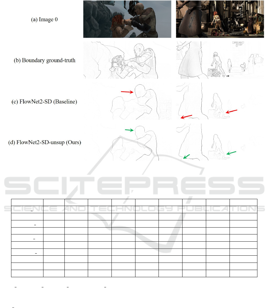
Figure 5: Visualization of motion boundaries from some Sintel validation sets. Our approach succeeds to detect more fine
structures (see green arrows) compared to the baseline.
Table 4: F-measure comparison between our motion boundary estimation generated by our method FlowNet2-SD-ft-unsup
using different loss function as described in Table 1 and the baseline on the Sintel train validation dataset.
f
1
f
2
f
3
f
4
f
5
f
6
f
7
Baseline
alley 2 Clean 0.7741 0.774 0.7744 0.774 0.7741 0.7746 0.7745 0.7733
Final 0.7736 0.7736 0.7736 0.7734 0.7735 0.7736 0.7736 0.7706
ambush 5 Clean 0.5029 0.5029 0.5027 0.5025 0.5027 0.503 0.5029 0.4675
Final 0.4665 0.4665 0.4665 0.4665 0.4665 0.4665 0.4665 0.4981
market 2 Clean 0.7324 0.7323 0.7324 0.7327 0.7324 0.7324 0.7324 0.6784
Final 0.6768 0.6767 0.6767 0.677 0.677 0.6768 0.6768 0.724
sleeping 1 Clean 0.2312 0.2318 0.231 0.2274 0.2309 0.2311 0.2312 0.2702
Final 0.3194 0.3196 0.3197 0.3202 0.3202 0.3195 0.3198 0.197
Average Clean 0.4077 0.4082 0.4078 0.403 0.4075 0.4078 0.4078 0.3435
Final 0.3736 0.3731 0.3737 0.3735 0.3735 0.3735 0.3735 0.3796
(alley 2, ambush 5, market 2 and sleeping 1) and in
some cases inside the same sequence Figure 6.
Figure 6 shows two different frames from am-
bush 5 validation dataset, their corresponding mag-
nitude maps for
~
U and
~
V and histogram of optical
flow magnitudes and EPE. The histogram of optical
flow magnitudes for the above frame shows that most
values have small magnitudes between -5 and 5 and
the majority are around zero with EPE 1.09. On the
other hand, the distribution of optical flow magnitudes
in the below frame are between -10 and 10 with ex-
tended distribution to 20 with EPE 10.095. This de-
notes that our method is not able to capture big dis-
placement in motion represented by high magnitude
values.
6 CONCLUSIONS
To conclude, we have introduced an unsupervised loss
function based on classical optical flow formula using
deep learning. Our approach shows potential to min-
imize the need of ground truth for both optical flow
estimation and motion boundary detection. Moreover,
benefit from pre-trained models to reduce time via fast
unsupervised fine-tuning. This work is opening the
Unsupervised Fine-tuning of Optical Flow for Better Motion Boundary Estimation
781
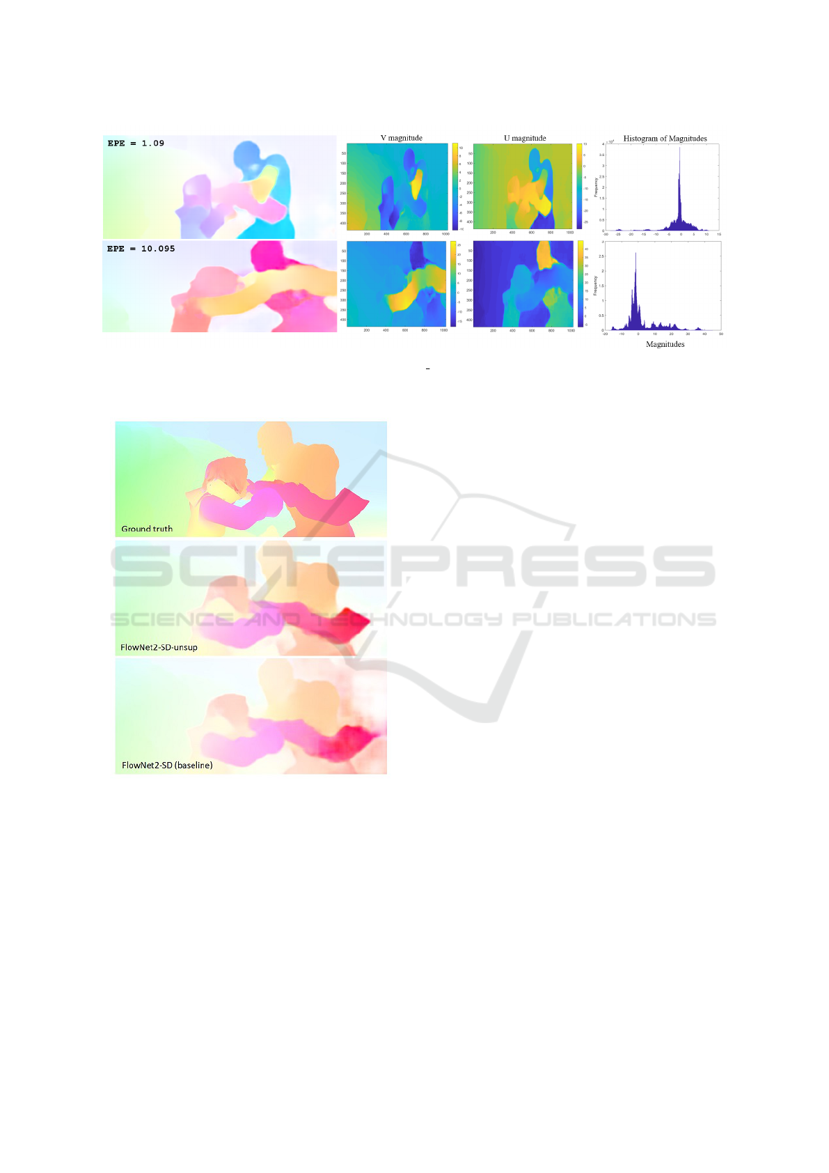
Figure 6: Two different images from validation sequence ambush 5 and their corresponding histograms of optical flow magni-
tudes and visualizations of magnitudes in U and V directions. It’s obvious that higher EPE value has higher large frequencies.
Figure 7: Qualitative results: We compare our results in the
second row using FlowNet2-SD-unsup with ground truth in
first row and the baseline generated from FlowNet2-SD in
the third row. Our model produces better flow and capturing
fine structures around boundaries.
opportunity to investigate more on how to enhance the
results to compete with state-of-the-art approaches.
One future work is handling large displacement which
tends to be a common draw back in many optical flow
estimators and reduce noise around edges.
REFERENCES
Alletto, S. and Rigazio, L. (2017). Unsupervised motion
flow estimation by generative adversarial networks.
Brox, T. and Malik, J. (2011). Large displacement optical
flow: descriptor matching in variational motion esti-
mation. IEEE transactions on pattern analysis and
machine intelligence, 33(3):500–513.
Butler, D. J., Wulff, J., Stanley, G. B., and Black, M. J.
(2012). A naturalistic open source movie for opti-
cal flow evaluation. In A. Fitzgibbon et al. (Eds.),
editor, ECCV, Part IV, LNCS 7577, pages 611–625.
Springer-Verlag.
Dosovitskiy, A., Fischer, P., Ilg, E., Hausser, P., Hazirbas,
C., Golkov, V., van der Smagt, P., Cremers, D., and
Brox, T. (2015). Flownet: Learning optical flow with
convolutional networks. In Proceedings of the ICCV,
pages 2758–2766.
Geiger, A., Lenz, P., and Urtasun, R. (2012). Are we ready
for autonomous driving? the kitti vision benchmark
suite. In CVPR.
Horn, B. K. and Schunck, B. G. (1981). Determining optical
flow. Artificial intelligence, 17(1-3):185–203.
Huang, G., Liu, Z., Weinberger, K. Q., and van der Maaten,
L. (2017). Densely connected convolutional networks.
In Proceedings of the IEEE conference on computer
vision and pattern recognition, volume 1, page 3.
Hui, T.-W., Tang, X., and Loy, C. C. (2018). Liteflownet:
A lightweight convolutional neural network for opti-
cal flow estimation. In Proceedings of the IEEE Con-
ference on Computer Vision and Pattern Recognition,
pages 8981–8989.
Ilg, E., Mayer, N., Saikia, T., Keuper, M., Dosovitskiy, A.,
and Brox, T. (2017). Flownet 2.0: Evolution of op-
tical flow estimation with deep networks. In CVPR,
volume 2.
Ilg, E., Saikia, T., Keuper, M., and Brox, T. (2018). Oc-
clusions, motion and depth boundaries with a generic
network for optical flow, disparity, or scene flow esti-
VISAPP 2019 - 14th International Conference on Computer Vision Theory and Applications
782

mation. In Proceedings of the European Conference
on Computer Vision (ECCV), pages 614–630.
Janai, J., Guney, F., Ranjan, A., Black, M., and Geiger, A.
(2018). Unsupervised learning of multi-frame optical
flow with occlusions. In Proceedings of the European
Conference on Computer Vision (ECCV), pages 690–
706.
Jason, J. Y., Harley, A. W., and Derpanis, K. G. (2016).
Back to basics: Unsupervised learning of optical flow
via brightness constancy and motion smoothness. In
European Conference on Computer Vision, pages 3–
10. Springer.
Long, G., Kneip, L., Alvarez, J. M., Li, H., Zhang, X., and
Yu, Q. (2016). Learning image matching by simply
watching video. In European Conference on Com-
puter Vision, pages 434–450. Springer.
Makansi, O., Ilg, E., and Brox, T. (2018). Fusionnet
and augmentedflownet: Selective proxy ground truth
for training on unlabeled images. arXiv preprint
arXiv:1808.06389.
Mayer, N., Ilg, E., Hausser, P., Fischer, P., Cremers, D.,
Dosovitskiy, A., and Brox, T. (2016). A large dataset
to train convolutional networks for disparity, optical
flow, and scene flow estimation. In Proceedings of
the IEEE Conference on Computer Vision and Pattern
Recognition, pages 4040–4048.
Menze, M. and Geiger, A. (2015). Object scene flow for
autonomous vehicles. In CVPR.
Papazoglou, A. and Ferrari, V. (2013). Fast object segmen-
tation in unconstrained video. In Proceedings of the
IEEE International Conference on Computer Vision,
pages 1777–1784.
Ranjan, A. and Black, M. J. (2017). Optical flow estimation
using a spatial pyramid network. In IEEE Conference
on Computer Vision and Pattern Recognition (CVPR),
volume 2, page 2. IEEE.
Ren, Z., Yan, J., Ni, B., Liu, B., Yang, X., and Zha, H.
(2017). Unsupervised deep learning for optical flow
estimation. In AAAI, volume 3, page 7.
Sun, D., Yang, X., Liu, M.-Y., and Kautz, J. (2018). Pwc-
net: Cnns for optical flow using pyramid, warping,
and cost volume. In Proceedings of the IEEE Con-
ference on Computer Vision and Pattern Recognition,
pages 8934–8943.
Wang, H., Kl
¨
aser, A., Schmid, C., and Liu, C.-L. (2013).
Dense trajectories and motion boundary descriptors
for action recognition. International journal of com-
puter vision, 103(1):60–79.
Wang, Y., Yang, Y., Yang, Z., Zhao, L., and Xu, W.
(2018). Occlusion aware unsupervised learning of op-
tical flow. In Proceedings of the IEEE Conference
on Computer Vision and Pattern Recognition, pages
4884–4893.
Wannenwetsch, A. S., Keuper, M., and Roth, S. (2017).
Probflow: Joint optical flow and uncertainty estima-
tion. In Computer Vision (ICCV), 2017 IEEE Interna-
tional Conference on, pages 1182–1191. IEEE.
Weinzaepfel, P., Revaud, J., Harchaoui, Z., and Schmid, C.
(2015). Learning to detect motion boundaries. In
The IEEE Conference on Computer Vision and Pat-
tern Recognition (CVPR).
Wulff, J., Butler, D. J., Stanley, G. B., and Black, M. J.
(2012). Lessons and insights from creating a synthetic
optical flow benchmark. In A. Fusiello et al. (Eds.),
editor, ECCV Workshop on Unsolved Problems in Op-
tical Flow and Stereo Estimation, Part II, LNCS 7584,
pages 168–177. Springer-Verlag.
Zhu, Y., Lan, Z., Newsam, S., and Hauptmann, A. G.
(2017). Guided optical flow learning. arXiv preprint
arXiv:1702.02295.
Unsupervised Fine-tuning of Optical Flow for Better Motion Boundary Estimation
783
