Roof Segmentation based on Deep Neural Networks

Regina Pohle-Fr¨ohlich

, Aaron Bohm

, P eer Ueberholz

, Ma ximilian Korb

and Ste ffen Goebbels

Institute for Pattern Recognition, Faculty of Electrical Engineering and Computer Science,

Niederrhein University of Applied Sciences, Reinarzstr. 49, 47805 Krefeld, Germany

Institute for High Performance Computing, Faculty of Electrical Engineering and Computer Science,

Niederrhein University of Applied Sciences, Reinarzstr. 49, 47805 Krefeld, Germany

Keywords:

Building Reconstruction, Deep Learning, Convolutional Neural Networks, Point Clouds.

Abstract:

The given paper investigates deep neural networks (DNNs) for segmentation of r oof regions in the context of

3D building reconstruction. Point clouds as well as derived depth and density images are used as input data.

For 3D building model generation we follow a data driven approach, because it allows the reconstruction of

roofs with more complex geometries than model driven methods. For this purpose, we need a preprocessing

step that segments roof regions of buildings according to the orientation of their slopes. In this paper, we test

three different DNNs and compare results with standard methods using thresholds either on gradients of 2D

height maps or on point normals. For the application of a U-Net, we transform point clouds to structured 2D

height maps, too. PointNet and PointNet++ directly accept unstructured point clouds as input data. Compared

to classical gradient and normal based threshold methods, our experiments with U-Net and PointNet++ lead

to better segmentation of roof structures.

1 INTRODUCTION

For a variety of simulation a nd planning applications,

3D city models are used. These models typically are

exchanged in the XML based description standard Ci-

tyGML. Each polygon represents a single wall, roof

facet or other building element according to the cho-

sen Level of Detail (LoD). Due to available data, most

CityGML models are given in LoD 2, i.e., they in-

clude roof and wall polygons but no further details

such as windows or doors. Often su ch models are ba-

sed on roof reconstruction using airborne laser scan-

ning or photogrammetric point clouds obtained from

oblique areal images. There are two main approaches

to roof reconstruction that might be used in combina-

tion on point clouds, cf. (Wang et al., 2018b): In the

ﬁrst approach model driven methods ﬁt parameterized

roof models to building sections. This lead s to simple

geometries. In some cases they differ signiﬁcantly

from the real roof layout because typica lly catalo-

gues of parameterized roof models are quite small.

In addition, parameters like slope mig ht be estima-

ted wrongly due to dormers or other small building

elements. The second approach is da ta driven, where

plane segments are ﬁtted to the point cloud and com-

bined to a watertight roof. This allows m odeling even

sophisticated r oof geometrie s that, for examp le , can

be found with churches. However, this appr oach is

sensitive to noise. Whereas ridge lin es can be de-

tected quite reliab ly by intersecting estimated planes,

step edges are difﬁcult to reconstruct if point clouds

are sparse, as in the case of airbo rne laser scanning, or

noisy, as in the case of photogrammetric point clouds.

In our previously developed data driven modeling

workﬂow (see (Goebbels and Pohle-Fr¨ohlich, 2016)

and subsequent papers), we ﬁrst segmented areas in

which the roof’s gradients homogeneously point into

the same direction. O nly within such areas, we then

used RANSAC to ﬁnd planes. Witho ut segmentation

prior to RANSAC, one would ﬁnd planes which might

be composed from many not con nected segments or

even planes that just cut larger structures. We com-

puted gradient directions on a he ight map. This is

a 2D greyscale image which is interpolated from the

z-coordinates of the point cloud. We used linear in-

terpolation on a Delaunay triangulation of the points.

Small gradients belong to ﬂat r oofs. Gradients with

length above a threshold value point into a signiﬁcant

direction. In order to gain segmentation we classi-

ﬁed these directions. Th ere are some shortcomings

with th is method: Classiﬁcation depends on compu-

ted threshold values. Moreover, to obtain the height

map we had to interpolate sparse or no isy point cloud

data. Results depend on the choice of resolution and

326

Pohle-Fröhlich, R., Bohm, A., Ueberholz, P., Korb, M. and Goebbels, S.

Roof Segmentation based on Deep Neural Networks.

DOI: 10.5220/0007343803260333

In Proceedings of the 14th International Joint Conference on Computer Vision, Imaging and Computer Graphics Theory and Applications (VISIGRAPP 2019), pages 326-333

ISBN: 978-989-758-354-4

the interpolation method. By interpolating, we lose

sharpness of ridge lines and step edges. In addition,

this is a 2D method. We cannot distingu ish between

points with same x- and y- coordinates that for exam-

ple occur with walls, chimneys, antennas or overhan-

ging trees.

Now the idea is to replace the segmentatio n step

by a deep neural network (DNN). In recent years,

DNNs have been applied successfully to many clas-

siﬁcation and even segmentation problems. DNNs

could be better suited to handle outliers due to anten-

nas and chimneys as well as occlusion by trees. Buil-

ding reconstruction algorithms typically use threshold

values that depend on point cloud density. DNNs

might be able to learn such th reshold values. Further-

more, due to normalization of input data, cloud den-

sity becomes less important.

However in contrast to images, point clouds are

unstructured, the amount of data is often much hig-

her, and there might be no color info rmation. Due to

the lack of structure, convolution of point clouds with

kernels is more elaborate tha n convolution of images.

Nevertheless, in rece nt years neural networks, also in-

cluding co nvolutional networks, have been developed

to directly work on point clouds.

In our paper, we evaluate 2D segmentation with

U-Net based on interpolated height m aps as well as

3D segmen ta tion directly on the point cloud with

PointNet and PointNet++. The tested networks clas-

sify 3D points to belong to six classes describing

walls, ﬂat roofs, roofs with a main slope facing north,

roofs with gradients pointing east, south and west. Fi-

nally, we compare the results with our previous met-

hods using thresholds either on the g radient values of

the 2D height ma p or on point normals.

2 RELATED WORK

DNNs are very popular in the area of computer vision

for object classiﬁcation an d semantic segmentation.

Especially, neural networks a re used for urban area

classiﬁcation with airborne laser scanning data ba sed

on height maps, see (Hu and Yuan, 2016; Yang et al.,

2017). In this context Boulch et. al. (Boulch et al.,

2017) used a neural network with encoder-decoder

architecture for segmentatio n of colored, dense point

clouds. They applied SegNet and U-Net for seman-

tic labelling . In our context, 2D segmentation of roof

regions can also be done on the previously described

height maps using U-Net (Ronneberger et al., 2015),

a convolutional DNN that has su ccessfully been ap-

plied to many image segmentation tasks. The U-Net

architecture consists of extraction and extension par ts

in which multi-channel fe ature maps are organized.

In the extraction part, featur e maps are connected to

realize either convo lutions or max pooling steps to

decrease the size and increase the number of featur e

maps. The expansion part of the network is sym-

metric to the extraction part and re a lizes convolution

steps, too. Here, instead of max pooling, upconvoluti-

ons are used to increase resolution. Additionally, high

resolution feature maps of the extraction part directly

contribute to up sampling steps. However, some of the

above mentioned shortcomin gs of working with 2D

height maps remain. Therefore, it seems to be a good

idea working directly on 3D data.

Generally, CNNs require structu red data. In the

most simple case, one can achieve this by rasteriza-

tion of point clouds and transfer into voxel represen-

tation. Unfortunately, this is memory and time con-

suming and might also imply the need of interpola-

tion. On this account, in most cases the resolution of

objects has to be decreased. A popular CNN for 3D

applications is VoxNet (Maturana and Scherer, 2015).

An alternative approach to structuring point

clouds is the use o f indexing structur e s. Input d a ta of

the Kd-network are kd-trees that are computed fro m

point clouds (Klokov and Lempitsky, 2017). Apart

from point’s coordinates, other p oint-wise attributes

can be considered. In OctNet (Wang et al., 2017) the

3D points are re presented with octre es. Typically, the

hierarchy of octants is only sparsely ﬁlled. 3D CNN

operations are performed only on octants occupied by

boundaries of the 3D shapes und er investigation. Due

to using index structures, both Kd-network and Oct-

Net are not rotation independ e nt. In addition , ge ne-

ration of index structures might be time consuming.

A further disadvantage ofthese methods is that new

convolution and pooling operations are necessary.

In recent ye a rs, deep learning methods for irregu-

lar data have been researched. One promine nt repre-

sentative is PointNet (see (Qi et al., 2017a)). In its ba-

sic form only the coordinate s of the points are used for

the classiﬁcation proce ss. PointNet processes every

point ide ntically and inde pendently in the ﬁrst step

with a T-Net. This network is a CNN w ith convolu-

tion layers, max pooling layers and two layers with

fully connected neurons. As a result, we receive a

transformed point cloud with uniform orien tation and

size, see Figure 1. In a next step, local features are

computed for every point.

Figure 1: The T-Net transforms the left input point cloud to

the aligned right point cloud.

Roof Segmentation based on Deep Neural Networks

327

In contrast to neighborhood relations, only glo-

bal positions of points are important for reco gnition

with PointNet. Since slopes of roo fs and vertex nor-

mals typically are obtained using nearest neighboring

points, this mig ht be disadvantageous with respect to

our application. PointNet’s successor PointNet++

(Qi et al., 2017b) appears to be be tter suited for this

task. PointNet++ is a multi-scale point-based network

that considers neighborhood information by applying

PointNet on nested partitioning of th e input point set.

In (Rethage et al., 2018) a hybrid a pproach for a

fully co nvolutional point network was chosen that is

based on multi-scale feature encoding by the use of

3D convolutions in combination with direct proces-

sing of the point clouds. The network runs on unorga-

nized input clouds and uses PointNe t as a low-level

feature descriptor. Internally, the input is transfor-

med into an ordered repr esentation. This transforma-

tion is followed by 3D convolutions to learn shape-

dependent relationships of the points at multiple sca-

les. With regard to semantic point segmentation, pu-

blished results are slightly worse than fo r PointNet++.

In their work (Hua et al., 2018) , Hua et. al pro-

posed a n ew convolution operator for CNN, called

point-wise convolution. This convolution operator

can be applied at each point in a point cloud to le-

arn point-wise features. Compared to other meth ods

which used Tensorﬂow’s optimized convolution o pe-

rators, running time was slower. According to (Hua

et al., 2018), per class segmentation accuracy was re-

ported to b e slightly worse than for PointNet.

In (Ben-Shabat et al., 2017) a 3D modiﬁed Fisher

vector was used as hybrid representation of the p oint

cloud. The 3D Fisher vector r epresentation describes

data samples from the point cloud in varying sizes by

their deviation from a Gaussian Mixture Model. Pu-

blished results obtained on a test data set were similar

to those of PointNet.

Furthermore, 3D data is often represented as a

mesh. Then a CNN for semantic segmentation can

be applied to a graph derived from the m e sh (Wang

et al., 2018a). In this case, special pooling operati-

ons are necessary to coarsen the graph. We we re not

able to use this method because automated mesh ge-

neration failed for a signiﬁcant number o f buildings.

Although so me points should become connected, dis-

tances between them were probably too large d ue to

outliers and shading effects.

Because of easy handling and good results in other

studies we did 3D segmentation with PointNet and

PointNet++. For comparison we also applied the U-

Net and classical gradient segmentation on 2D h eight

maps.

3 TRAINING DATA

DNNs require a huge amount of training d a ta . We di-

rectly obtaine d ground truth by sampling point clouds

from alrea dy existing 3D city models and received an-

notations at nearly no cost by mapping face normals

to our six classes,

Wall

Flat Roof

North

South

East

and

West

We worked with a 3D mo del of four square kilo-

meters of the center of the city of Krefeld tha t consists

of more than 10,000 buildings. We converted each

single CityGML building model into OBJ-format re-

presentation such that each triangle had a label (color)

referrin g to its ro of or wall polygon. Per deﬁnition,

each building’s ground plane lay in the x-y-plan e . Ad-

ditionally, we rotated the buildings re presentation in

such way that the largest edge of the building ’s ca-

dastral footprint pointed into th e direction of x-axis of

the coordinate system. We the n scaled the model to

ﬁt within the cube [−1, 1]× [−1, 1] ×[−1, 1]. By allo-

wing three different component-wise scaling factor s,

directions of normals did change slightly. This was

tolerable because, as a preprocessing step to plane es-

timation, we still got useful segmentation into roof’s

gradient directions. If we did not scale to comple-

tely cover the interval [−1, 1] in all three dimensions

then PointNet’s preprocessing step performed geome-

tric transformatio ns that changed classiﬁcation.

With the too l CloudCompare, we randomly sam-

pled 2048 or 4096 labeled surface points for efﬁcient

processing of the da ta by PointNet. To obtain ground

truth, we computed face normals of all wall a nd roof

planes belonging to th e transformed building model,

see Figure 2. According to the normals, we classi-

ﬁed the planes into the classes

Wall

(z-component of

normal is zero),

Flat Roof

(x- and y- components

of normals are (approximately) zero),

North

(roofs

with slope to the north, i.e. in direction of the po-

sitive y-axis),

East

(positive x-axis),

South

(nega-

tive y-axis) and

West

(negative y-axis). According

to the points’ labels, we annotated them with their

Figure 2: Distribution of face normals of roof and wall pla-

nes (left) and point normals obtained from t he point neig-

hbors (right): The normals were projected to the x-y-plane

by removing their z-coordinate. E ach dot represents the

normal vector associated with a point of the cloud. Cle-

arly, four major directions are visible, denoted as classes

North

East

South

and

West

in this paper. Normals of ﬂat

roofs were marked in blue, white pixels represent normals

of walls.

VISAPP 2019 - 14th International Conference on Computer Vision Theory and Applications

328

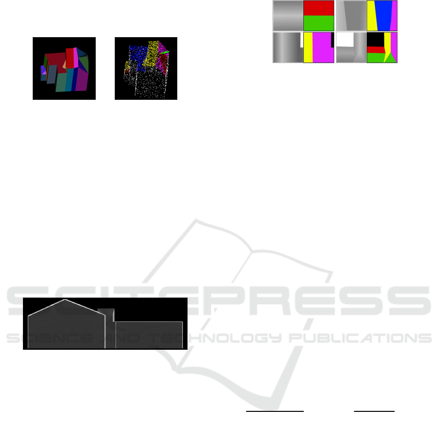
correspo nding class, see Figure 3. We ensure that

all classes contain approximately the same number of

points. PointNet++ allows for additional point-wise

Figure 3: Left: 3D model of the building, each facet is mar-

ked with a different color. Right: Ground tr uth classiﬁcation

of a building’s point cloud; Facets with different slope but

same gradient direction are not distinct.

input data, and PointNet can be executed with de ri-

ved data instead of original points. To this end, we

equippe d the points with point (vertex) normals com-

puted from their nearest neig hbors. Only for network

training w e additionally considered face normals. A

point’s face normal is the normal vector of the buil-

ding’s plane that is associated with the point Also,

we generated multi-view density images by orthogo -

nally projecting all points to the x-y-, x-z− and y-z-

planes, see Figu re 4. Such density maps were already

used for o bject classiﬁcation in (Minto et al., 2018).

On each plane, w e ac cumulated the num ber of points

Figure 4: Density image on the x-z-plane.

using a 256 × 256 raster. Thus, the data set contains

3D points, two (often different) cor respondin g normal

vectors and also triples of density values accor ding to

a point’s positions in the three r aster images.

For the application of U-Net on h eight maps, we

again turned each building so that the longest foot-

print edge matched the x-axis. Then, we initialized a

greyscale height map image covering the buildings’s

footpr int with height values taken fro m z-coordinates

of the point cloud. We completely ﬁlled the ima ge

using linear interpolation, see greyscale pictures in

Figure 5. This served as the net’s inpu t. To ﬁnd cor-

respond ing ground truth segmentation, we used the

face norm a ls of triangles from the building model,

which were projected into the x-y-plane. If a pixel

was outside a building’s footprint then we classiﬁed it

as backgro und.

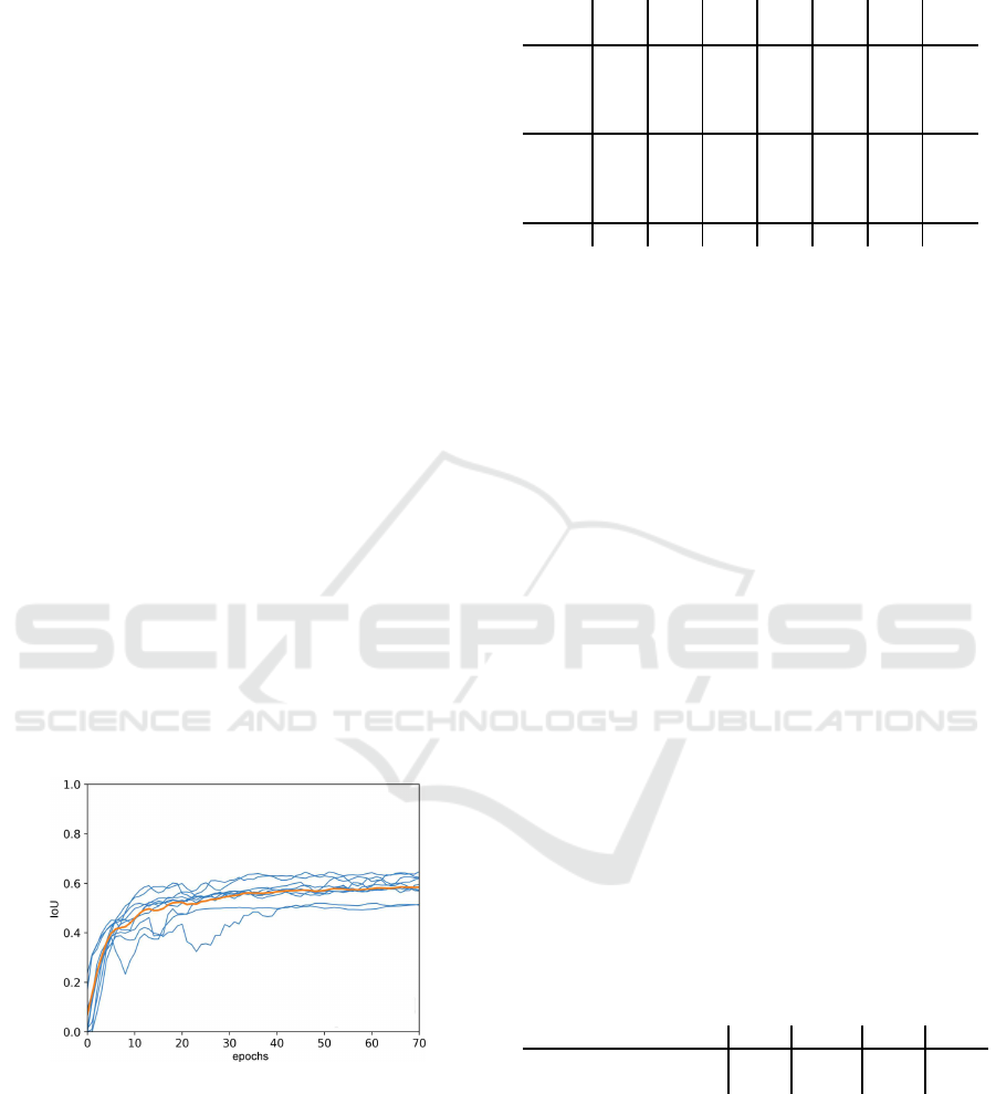
Figure 5 shows examples for height maps and as-

sociated ground truth maps. The class

Wall

is not

included in ground truth maps because walls are co-

vered by roof poin ts.

Figure 5: Height maps with ground tr uth annotation: blue

regions represent ﬂat roofs, black areas do not belong to the

building, the other colors r epresent the classes

North

East

South

and

West

We used data derived from existing building mo-

dels both for training and testing . Thus, we trained

the network with 90% of sampled buildings and used

10% as test da ta . Because of computing time, we did

not apply cross-validation. But we checked that the re

is no over-ﬁtting. Also, the ratio 90% : 10% led to

best recognition results. However, in order to evaluate

networks’ performance on real point clou ds obtained

by airborne laser scan ning, we extracted the points of

21 buildings from such a cloud. Then we removed

outliers because such points do not occur in training

data. Finally, we manually classiﬁed the points.

4 EXPERIMENTS

To measure quality of results, we use the established

intersect over union metric (IoU). For a given class

and a given building, TP (true positive) is the num -

ber of points or pixels that are correctly identiﬁed as

being members of this class: TN ( true negative) is

the number of input po ints that are co rrectly classi-

ﬁed as not belonging to the given class. In turn, FP

(false positive) and FN (false negative) a re numbers of

wrongly classiﬁed points. Then pr ecision is deﬁned

via

TP + TN

TP+ TN+FP + FN

and IoU :=

TP + FP + FN

. The num-

ber TN does not occur in this deﬁnition because in

general most p oints do belong to other c lasses (back-

ground) and one wants to avoid a good rating for net-

works that just classify backgro und. To get a qua-

lity measure for a given class and all buildings of the

test data set, we restrict ourselves to those buildings

only, that include this class according to ground tr uth.

For e a ch of the se buildings, we separately compute

an IoU value and then determine the arithmetic mean

over all such buildings. We do not set IoU := 1 if a

class is not contained in a building’s ground truth as

it is done in PointNet. Thus, presente d IoU-values

might be smaller but more meaningful than measured

with unchanged PointNet code. Because of compu-

ting IoU values separately for each building and not

weighting with the building’s class size, we amplify

errors of small classes.

Roof Segmentation based on Deep Neural Networks

329

4.1 U-Net on Height Maps

We applied U-N e t to 25,000 patches of 2,800 greys-

cale height maps with varying parameters. Each

height map was an image with 492 × 492 pixel.

All tests were perform ed using cro ss e ntropy error

function. Nets might learn trainin g data very well but

fail with other input data. This effect is called overﬁt-

ting. To avoid overﬁtting, we generally used regula-

rization by adding a constant fraction of the absolute

sum of the net’s weights to the error fun c tion.

We selected the Adam optimizer (Kingma and

Adam, 2015) as a statistical gradient descent method.

We also tested with Adagrad (Duchi et al., 2011) and

RMSProp but, as expected, the Adam method perfor-

med best by far. It reached high IoU values around

0.8 within 1 5 epochs in some initial tests. Simple

gradient descent and Adagrad optimizer did not re-

ach values above 0.3 after 200 epochs, and RMSProp

tended towards a decrease in IoU after 100 epochs.

We worked with a learning rate of 0.0001, as

smaller rates did not yield better IoU results after the

same nu mber of epochs. To the contrast, hig her rates

resulted in signiﬁcantly smaller I oU numbers.

We initialized the nets with random weights fol-

lowing a Gaussian distribution. Thus it was desirable

to get stable results independen t o f the initial values.

By repeating experiments ten times under same con-

ditions, we tested stability. Thereby, we observed two

outliers with IoU values that were about 20% lower

than the values obtained for the other eight experi-

ments within the same ma gnitude, see Figur e 6.

Figure 6: IoU values for learning class

Flat Roof

with U-

Net: Blue curves belong t o independent trainings with same

net conﬁguration, orange curve shows arithmetic mean.

Stability can be improved either by using the dro-

pout metho d (that was applied in previously me ntio-

ned stability tests) or batch normalization. But both

methods should not be used at the same time, cf. (Li

et al. , 2018). With stable networks, all further results

were obtained using a single set of initial weights.

Table 1: IoU values aft er 200 training epochs: Numbers in

the ﬁrst column refer to the amount of activated neurons.

drop-

Flat North East South West

back- arith.

out

Roof

round mean

full

90% 66.8%86.1%90.2%88.0%93.9%98.6%87.3%

80%

59.7% 80.3% 88.6% 81.0% 91.6% 98.5% 83.3%

70%

59.2% 76.3% 87.2% 76.9% 89.4% 98.5% 81.3%

half

90% 61.5% 83.0% 90.0% 83.4% 92.3% 98.5% 84.8%

80%

56.3% 78.5% 88.3% 78.1% 90.5% 98.4% 81.7%

70%

52.0% 70.4% 84.6% 71,3% 86.5% 98.4% 77.2%

no 60.3% 82.2% 89.2% 81.5% 92.1% 98.4% 84.0%

By using the dropout method, a predeﬁned n um-

ber of randomly chosen neurons are deactivated. The

desired effect is that results become more robust and

not dependent on single neurons. We analyzed two

different conﬁgurations. In the “full dropout” variant,

dropout was applied to all convolution layers. The

“half d ropout” conﬁguration applied dropout to every

second convolution layer starting with the ﬁrst. Table

1 shows that a 90% “full dropout” performed best,

i.e., 10% of neurons were randomly deactivated.

The ne tworks were trained with data grouped into

batches. For each activation la yer’s input, batch nor-

malization subtracts the batch’s me a n and divides the

result by the batch’s standa rd deviation. It also mul-

tiplies it with a trainable parameter γ and adds anot-

her trainable parameter β such th at gradient descent

can modify them in stead of having to change many

weights. As expec ted, with batch normalization, IoU

values were higher for all tested learning rates than

without use of batch normalization and dropout. With

dropout, IoU numbers were alike, but variance was

greater (cf. Figure 6) , thus stability was worse.

The architecture of U-Net allows modiﬁcation of

two speciﬁc parameters: The number of top-layer fe-

ature maps a nd the size of the convolution kernel. Ta-

ble 2 shows the r esults of four trainings that only dif-

fer in the number of feature maps. Due to running

time, we decided to work with 16 feature maps. We

Table 2: Inﬂuence of the number of t op-level feature maps.

number of feature maps

32 16 8 4

running time 23h 11.8h 5.2h 2.7h

median IoU

85% 83% 62% 48%

applied 3 × 3 and 5 × 5 kernels and found that, with

using batch normalization, 5 × 5 kernel led to equally

good IoU values as 3 × 3 kernel with 90% “full dro-

pout” or with batch normalization. But due to the lar-

ger kernel size, less convolution layers were n e eded,

and running time decreased by about 30%.

We compare U-Net results with following classi-

cal segmentation approach on the 2D greyscale height

map in Table 3: On the height map, we computed gra-

VISAPP 2019 - 14th International Conference on Computer Vision Theory and Applications

330

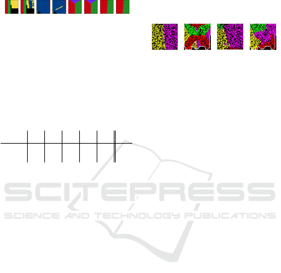
Figure 7: Ground truth and prediction: Black pixel are

background, blue denotes

Flat Roof

dients via convo lution with 3 × 3 or 5 × 5 Sobel ker-

nel. Pixels belongin g to gradients with length below a

threshold value 0.1 were classiﬁed to be part of a ﬂat

roof. Otherwise, a gradie nt’s direction in x-y-plane

determines the class

North

East

South

West

. U-

Net clearly leads to b etter segmentation results than

thresholding of gradients computed with Sobel ker-

nels. Figure 7 compares ground truth with network

results. The image pairs in the upper row show quan-

tization errors in areas with low slop e.

Table 3: IoU values achieved with U-Net in comparison to

classical segmentation.

Flat North East South West

arith.

Roof

mean

U-Net 72.8 94.6% 93.2% 94.5% 90.9% 89.2%

3 × 3 Sobel

84.4% 77.4% 65.4% 73.8% 65.8% 73.4%

5 × 5 Sobel

80.6% 81.1% 72.2% 78.1% 72.4% 76.9%

4.2 PointNet

PointNet is design ed only to handle point clouds in

which each point consists of three coordinate va-

lues. We evaluated both, with the points’ x- y- and z-

coordinates but also with replacing the three values by

the components of co rrespond ing vertex normal vec-

tors that are computed from the point’s nearest neig-

hbors. Face normals typically are not available as in-

put and were only used to deﬁne ground truth.

To select parameter values, we trained the ne twork

with the points’ coordina te s. We chose the learning

rate 0.001 that, with regard to IoU, perf ormed as well

as lower rates 0.0005 and 0.0001, wherea s higher ra-

tes 0.01 and 0.005 resulted in signiﬁcantly lower IoU

values. The choice of using batch normalization im-

proved results slightly.

With in PointNet, T-Net serves as a pr eprocessing

step. This step can be followed by a similar T-Net-

Feature network. We observed slight improvements

in all tests when choosing to use both transformations.

Probably, the improvement was only small because

our input data was rotated according to the longest

footpr int edge. Hence, a suitable transformation was

in place alre a dy.

With regard to stability, by repeating a training

with random initial weights an d batch normalization

we did not observe outliers as we did for U-Net tests

based on the dropout method. However, Table 4 and

Figure 8 show that PointNet did not perform well.

The number of wall points was higher than the num-

ber of points in other classes. Therefo re, wall points

were classiﬁed better.

Figure 8: Two examples of ground truth segmentation (left)

and prediction (right) with PointNet on x, y, z coordinates.

One would expect that results should improve if

points were replaced with their corresponding point

normal vectors. The direction of a normal vector im-

mediately implies the class. Only differences between

face norm a ls (used to determine ground truth) and

point normals should lead to errors. With exception

of class

West

, PointNet applied to point nor mals in-

deed yields better but still not convincing results, see

Ta ble 4. Applyin g trained networks to manually clas-

siﬁed real point clouds changed results for the worse.

4.3 PointNet++

In contrast to PointNet, its successor PointNet++

accepts six values per point as input. That allowed

evaluating PointNet++’ performance with two very

different inputs: We used 3D points in connection

with normal vectors as well as 3D points in combina-

tion with three projected density values, see Section

3. Since face normals can be generated only from 3D

building models and not from point clouds directly,

we tested ou r conﬁgurations with point normals. Any-

how, for training the n e tworks with mode l data we can

use either point normals or face normals detected on

planes, see Figure 9. Tab le 5 summarizes correspon-

ding results. All class sizes were chosen to be ap-

proxim ately e qual for training but not for testing with

real world data. It is not surprising that the network

performs b e tter, if training and test data matched, i.e.,

one should train with point normals. This also holds

true for testing with real world data. However, seg-

mentation results were a good deal poorer, see Table

6. Independent of chosen segmentation method, IoU

values of walls were low. That is due to the fact that

in airborne laser scanning data walls are mostly invi-

sible. Thus, only 3% of points belong to walls.

PointNet++ trained on point normals and tes-

ted on model data even perf ormed signiﬁcantly better

than outcomes of classical point norm a l-based seg-

mentation using thresho ld values (Table 5). In this

situation the network apparently learne d thresholds

more easily. In case of real world point clouds, the

picture was not as clear (see Table 6). Reality an d le-

arning da ta seemed to differ too much, e.g., r eal roofs

Roof Segmentation based on Deep Neural Networks

331

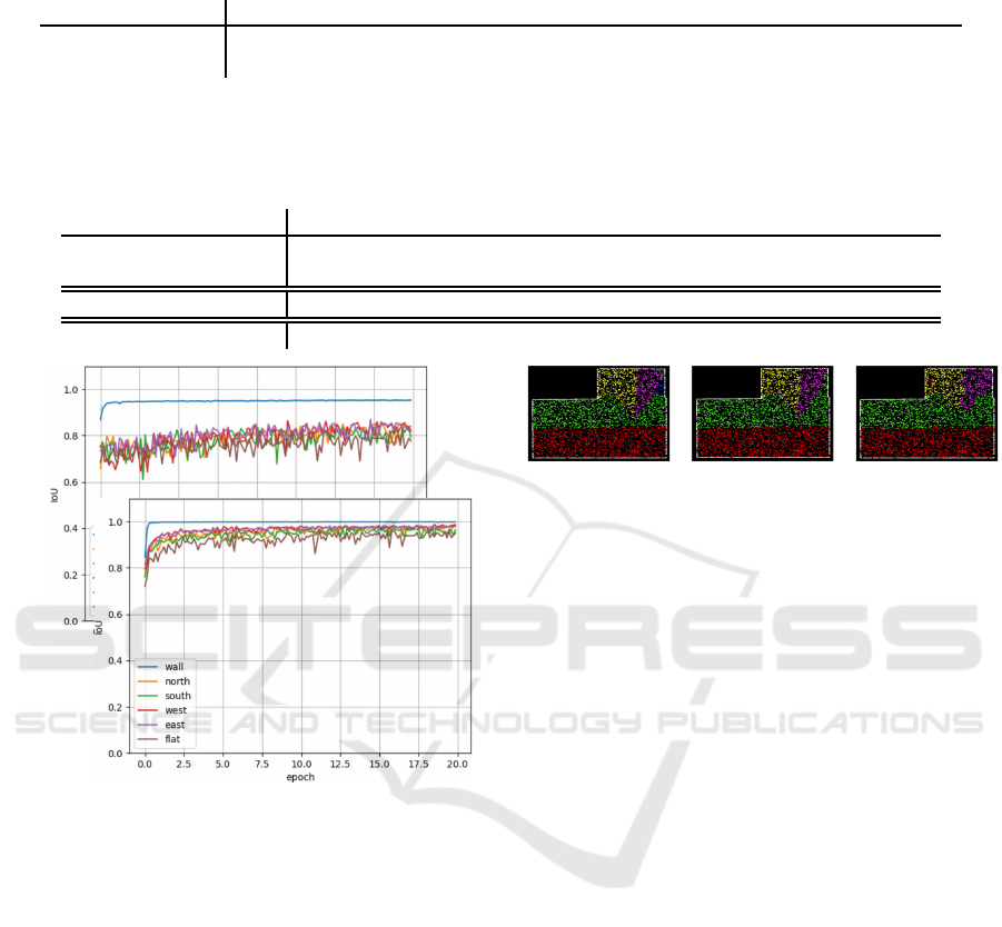
Table 4: On the one hand, PointNet was trained and tested with points and on the other hand the network was trained and

tested with point normals. For comparison, IoU values of classical segmentation are given in Table 5.

training variant

Wall North East South West Flat Roof

arithmetic mean

x, y, z coordinates 69.4% 34.8% 31.8% 27.3% 25.1% 34.9% 37.2%

point normals

92.5% 50.1% 33.7% 51.1% 18.4% 75.7% 53.6%

Table 5: PointNet++ trained over 200 epochs and t ested with points and normals of generated data as well as with density

values from three points of view: To train the network with normals, we either used point or face normals obtained from

90% of 3D models. For testing on remaining 10% of models, points were equipped with point normals. For comparison, IoU

values of segmentation on point normals (using same thresholds as for ground truth generation on face normals) are listed.

training variant

Wall North East South West Flat Roof

mean

point normals 96.3% 84.3% 83.5% 84.1% 83.5% 84.6% 86.1%

face normals

88.1% 7 0.8% 74.6% 68.3% 73.8% 69.5% 74.2%

density data 95.1% 85.4% 84.7% 85.9% 85.4% 85.9% 87.1%

classical segmentation 88.1% 69.8% 76.6% 69.9% 76.6% 68.8 % 74.9%

Figure 9: IoU values during training on points and normal

vectors with PointNet++: Upper plots belong to training

with point normals. Second plots summarize training with

face normals.

were not exactly planar.

When applying PointNet++ with point co ordina-

tes and three corresponding density values instead of

normals r esults were similar good than for training

with point norma ls. Both variants were better than

results for training with face normals, see Table 5.

Ridge lines and step edg e s were clearly visible in den-

sity images. But surprisingly, segmenta tion results al-

ong these lines appe a red noisier when using den sity

values than point normals, see Figure 10.

5 CONCLUSION

Deep learning shows potential to improve existing al-

gorithms for 3D building reconstruction. Both U-Net

Figure 10: Difference between PointNet++ segmentation

based on point normals and segmentation on density values:

ground truth (left), point normal segmentation (middle),

density value segmentation (right). To avoid error coming

from e.g. small dormers higher resolution is required. This

can be obtained by splitting up buildings into parts, cf. Fi-

gure 11.

trained on height maps and, if trained o n point nor-

mals or density images, PointNet++ are able to yield

better segmentation results than we c ould obtain with

classical gradient or normal based approaches. At le-

ast this holds true for testing with point clou ds that are

sampled from 3D city models. For application to real

world point clouds, we have to im prove our training

data. Recently, we trained with an notated real 3D data

and got similar results as on training data described in

this paper.

In ou r tests, 3D networks did not perform better

than 2D U-Net. Again, the main reason might be that

our trainin g data for roofs can be represented in 2.5D.

Most non-ﬂat roofs possess only four main gra-

dient dir ections. Therefore, classiﬁcation into ﬂat

roofs and four direc tions generally serves well. Ho-

wever, in future work we will increase the number of

classes to improve segmentation results for sophisti-

cated roof topologies. To this end , we also have to

split up buildings into small processable parts instead

of using non-uniform scaling. This also solves the

problem that our cu rrently used networks o nly accept

quite small point clouds due to memory restrictions.

As tested with PointNet++, segmentation results o f

parts can be merged without signiﬁcant loss of qua-

lity, see Figur e 11. Suitable strategies for split-up pro-

cedures have to be developed.

VISAPP 2019 - 14th International Conference on Computer Vision Theory and Applications

332

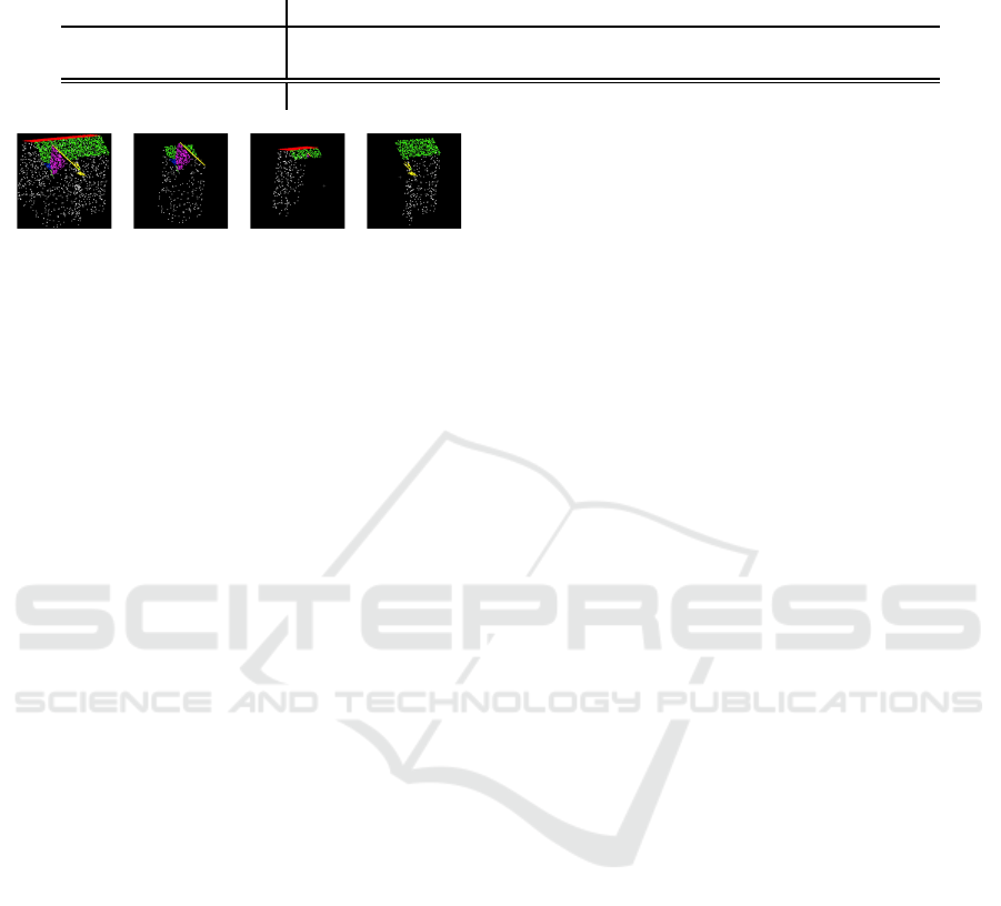
Table 6: PointNet++ tested with real world point clouds: To train the network, w e either used point or face normals obtained

from 90% of 3D models as in Table 5. For testing, we used real point clouds equipped with point normals. Results were

compared with classical threshold segmentation as in Table 5.

training variant

Wall North East South West Flat Roof

mean

point normals 65.2% 64.3% 52.0 % 70.7% 56.8% 55.7% 60.8%

face normals

53.3% 5 6.2% 57.0% 73.2% 57.1% 47.1% 57.3%

classical segmentation 52.1% 60.3% 59.5% 71.6% 59.4% 44.2% 57.9 %

Figure 11: Stable segmentation results on cloud subsets.

ACKNOWLEDGEMENT

This work was supported by a generous hardware

grant from NVIDIA.

REFERENCES

Ben-Shabat, Y., Lindenbaum, M., and Fischer, A.

(2017). 3D point cloud classiﬁcation and segmenta-

tion using 3D modiﬁed ﬁsher vector representation

for convolutional neural networks. arXiv preprint

arXiv:1711.08241.

Boulch, A., Le Saux, B., and Audebert, N. ( 2017). Un-

structured point cloud semantic labeling using deep

segmentation networks. In 3DOR.

Duchi, J., H azan, E., and Singer, Y. (2011). Adaptive

subgradient methods for online learning and stochas-

tic optimization. Journal of Machine Learning Rese-

arch, 12:12:2121–2159.

Goebbels, S. and Pohle-Fr¨ohlich, R. (2016). Roof recon-

struction from airborne laser scanning data based on

image processing methods. ISPRS Ann. Photogramm.

Remote Sens. and Spatial Inf. Sci., III-3:407–414.

Hu, X. and Yuan, Y. (2016). Deep-learning-based classiﬁ-

cation for dtm extraction from als point cloud. Remote

sensing, 8(9):730.

Hua, B.-S., Tran, M.-K., and Yeung, S.-K. (2018). Point-

wise convolutional neural networks. In Proceedings of

the IEEE Conference on Computer Vision and Pattern

Recognition, pages 984–993.

Kingma, D. and A dam, J. B. (2015). A method for stochas-

tic optimization. In International Conference on Le-

arning Representations, pages 1–15, San Diego, CA.

Klokov, R. and Lempitsky, V. S. (2017). Escape from cells:

Deep kd-networks f or the recognition of 3D point

cloud models. 2017 IEEE International Conference

on Computer Vision (ICCV), pages 863–872.

Li, X., Chen, S., Hu, X., and Yang, J. (2018). Understan-

ding the disharmony between dropout and batch nor-

malization by variance shift. CoRR, abs/1801.05134.

Maturana, D. and Scherer, S. (2015). Voxnet: A 3D convo-

lutional neural network for real-time object recogni-

tion. In Intelligent Robots and Systems (IROS), 2015

IEEE/RSJ International Conference on, pages 922–

928. IEEE.

Minto, L., Zanuttigh, P., and Pagnutti, G. (2018). Deep

learning for 3d shape classiﬁcation based on volume-

tric density and surface approximation clues. In VISI-

GRAPP (5: VISAPP), pages 317–324.

Qi, C. R., S u, H., Mo, K., and Guibas, L. J. (2017a). Point-

net: Deep learning on point sets for 3D classiﬁcation

and segmentation. In Proceedings of the IEEE Con-

ference on Computer Vision and Pattern Recognition

(CVPR), pages 77–85.

Qi, C. R., Yi, L., Su, H., and Guibas, L. (2017b). Point-

net++: Deep hierarchical f eature learning on point

sets in a metric space. In Proceedings of the 31st

Conference on Neural Information Processing Sys-

tems (NIPS).

Rethage, D., Wald, J., Sturm, J., Navab, N., and Tombari, F.

(2018). Fully-convolutional point networks for large-

scale point clouds. arXiv preprint arXiv:1808.06840.

Ronneberger, O., Fi scher, P., and Brox, T. (2015). U-net:

Convolutional networks for biomedical image seg-

mentation. CoRR, abs/1505.04597.

Wang, P., Gan, Y., Shui, P., Yu, F., Zhang, Y., Chen, S., and

Sun, Z. (2018a). 3D shape segmentation via shape

fully convolutional networks. Computers & Graphics,

70:128–139.

Wang, P.-S., Liu, Y., Guo, Y.-X., Sun, C .-Y., and Tong, X.

(2017). O-CNN: Octree-based convolutional neural

networks for 3D shape analysis. ACM Transactions

on Graphics (TOG), 36(4):72:1–72:11.

Wang, R., Peethambaran, J., and Dong, C. (2018b). Li-

DAR point clouds to 3D urban models: A review.

IEEE J. Sel. Topics Appl. Earth Observ. Remote Sens.,

11(2):606–627.

Yang, Z., Jiang, W., Xu, B., Zhu, Q., Jiang, S., and Huang,

W. (2017). A convolutional neural network-based 3D

semantic labeling method for als point clouds. Remote

Sensing, 9(9):936.

Roof Segmentation based on Deep Neural Networks

333