Uncertainty-aware Prediction in Spatio-temporal Simulation Ensemble

Visualizations

Marina Evers and Lars Linsen

Westf

alische Wilhelms-Universit

at M

unster, Germany

Keywords:

Uncertainty Visualization, Ensemble Visualization, Parameter-Space Visualization, Volume Visualization.

Abstract:

Spatio-temporal simulation ensembles are used to investigate the dependence of the simulation behavior on

input parameters. Running simulations for a large number of input parameter settings is computationally ex-

pensive. We propose a scheme for exploring the parameter space using predictions of simulation outcomes and

estimating the uncertainty in the predictions. The prediction approximates the simulation result by interpolat-

ing feature vectors of existing runs. The feature vectors are used to compute similarities between simulation

runs facilitating visualization of the entire ensemble within a 2D (or 1D-over-time) multi-dimensional scaling

embedding. Uncertainties of the prediction are computed based on distance, interpolation and diversity, which

are visually encoded by an uncertainty band in the embedding. To guide the user to choose suitable parameter

settings for prediction, we also propose a parameter-space visualization of the uncertainty. The approach is

applied to real-world data simulating deep-water impact of asteroids.

1 INTRODUCTION

Spatio-temporal ensemble visualizations are common

in many areas of science like physics or geography.

These simulations typically depend on initial condi-

tions or input parameters. To understand the depen-

dence of the simulation result on the initial parame-

ters, it is commonly necessary to create an ensemble

including various simulation runs.

Visualizing an ensemble comes with the challenge

of handling large amounts of data and establishing a

visual encoding that allows for the comparative analy-

sis of simulation runs. Another challenge inherent to

ensembles is to determine, which parameter settings

to choose for desirable simulation outcomes. We pro-

pose an approach that facilitates the analysis of the pa-

rameter space of spatio-temporal simulation ensem-

bles by predicting simulation outcomes of new pa-

rameter settings from existing ones. The method is

computationally inexpensive as it is based on the in-

terpolation of feature vectors, see Section 4. The pre-

dicted result is visualized within the embedding pro-

posed by Fofonov et al. (Fofonov et al., 2016), see

Section 3.

It is important to visually convey how good we

expect the prediction to be. Thus, we compute the

uncertainty of the prediction based on multiple fac-

tors such as distance to existing settings in the pa-

rameter space, the uncertainty introduced by the in-

terpolation scheme, and the diversity of the existing

results used for interpolation, see Section 5. We vi-

sualize the uncertainty in the form of an uncertainty

band in the embedding. Moreover, we visualize the

uncertainty of possible predictions in the parameter

space, which facilitates choosing suitable parameter

settings for prediction (and eventually for running the

actual simulation) in the sense of computational steer-

ing, see Section 6.

We apply our approach within a real-world sce-

nario of investigating the inﬂuence of multiple input

parameters on the result of an ensemble of deep water

impact by asteroid simulations, see Section 7.

2 RELATED WORK

Many visualization approaches for spatio-temporal

simulation ensembles display statistical information

such as mean or variance of the ensemble (Potter

et al., 2009) (Sanyal et al., 2010), which does not sup-

port the comparative analysis of individual simulation

runs nor the analysis of the inﬂuence of simulation pa-

rameters. Phadke et al. (Phadke et al., 2012) proposed

techniques to explore and compare ensemble mem-

bers, but they are limited to small numbers. Fofonov

et al. (Fofonov et al., 2016) introduced the concept

216

Evers, M. and Linsen, L.

Uncertainty-aware Prediction in Spatio-temporal Simulation Ensemble Visualizations.

DOI: 10.5220/0007344702160224

In Proceedings of the 14th International Joint Conference on Computer Vision, Imaging and Computer Graphics Theory and Applications (VISIGRAPP 2019), pages 216-224

ISBN: 978-989-758-354-4

of multi-run plots that allows for visualizing simulta-

neously the temporal evolution of all simulation runs

within an ensemble. We will build upon this idea, see

Section 3. Applications of the multi-run plot include

the visual representation of ensembles to detect pat-

terns and outliers (Fofonov and Linsen, 2018a). Our

goal is to predict the outcome of new simulation runs

and determine their uncertainty. Fofonov et al. nei-

ther provide information beyond the scope of the sim-

ulated run nor do they support choosing parameters

for further simulation runs. Different tools for compu-

tational steering exist in the analysis of ensemble data

such as World Lines (Waser et al., 2010) and ComVis

(Matkovic et al., 2008). Splechtna et al. (Splechtna

et al., 2015) introduced an interactive visual analy-

sis with hierarchical steering that supports multi-level

simulation models. However, these approaches are

only applicable if the computation of a simulation run

does not take too much time.

To obtain a better understanding of the relation-

ship between the parameter space and the target space

in an interactive setting, Berger et al. (Berger et al.,

2011) proposed a method using statistical learning to

predict further results and apply it to car engine de-

sign. In the following years, Sedlmair et al. (Sedlmair

et al., 2014) provided an abstract conceptual frame-

work. Potter et al. (Potter et al., 2017) proposed an

ensemble steering framework similar to the concep-

tional framework that uses approximations of simu-

lations based on machine learning to explore, design,

and plan energy systems. They also mention the pos-

sibility of a later simulation to eventually produce

a more accurate result. None of the mentioned ap-

proaches for parameter space visualization deals with

multi-run spatio-temporal simulation ensembles that

are common for physical simulations, which is what

we are addressing in this paper.

Recently, there has been active research on the vi-

sualization of uncertainty, cf. (Pang et al., 1997) (Gri-

ethe and Schumann, 2006) (Potter et al., 2012) (Liu

et al., 2017)(Rhodes et al., 2003)(Xie et al., 2015).

Some of them are within the context of simulation

ensembles such as Noodles (Sanyal et al., 2010) or

EnsembleVis (Potter et al., 2009) for analyzing the

associated uncertainty in the data. Both tools as-

sign the uncertainty by computing the standard de-

viation (or variance) to the means using statistically

pre-processed data. We, instead, propose novel ap-

proaches for estimating uncertainty in the parameter

space and respective visualizations and for prediction

outcomes in the embedded space.

3 BACKGROUND

Multi-run Plot. Our approach is based on the visual

representation of the simulation ensemble within an

embedding as proposed by Fofonov et al. (Fofonov

et al., 2016). Each simulation run is depicted as a

curve parametrized over time, where positions on the

curve reﬂect similarities of the time steps of the runs.

To compute the multi-run plots, Fofonov et al. (Fo-

fonov et al., 2016) propose to compute the similarity

of two scalar ﬁelds by computing the Jaccard distance

of the volumes that are enclosed by the isosurfaces

of a representative isovalue. They later generalize

this isosurface similarity measure to a ﬁeld similar-

ity measure, which does not require the choice of a

representative isovalue, and even to a multiﬁeld simi-

larity measure that simultaneously considers multiple

ﬁelds (Fofonov and Linsen, 2018b). We support all

options for similarity measures.

In case of the isosurface similarity, the values at

the samples are thresholded against the isovalue lead-

ing to a binary n-dimensional vector, where n is the

number of samples. In the case of ﬁeld similarity, the

ﬁeld values are stored in the n-dimensional vector. We

refer to this vector as feature vector and will use it for

our predictions, see Section 4.

The multi-run plot is generated by using pair-

wise dissimilarities of all time steps of all simula-

tion runs, which are stored in a distance matrix. The

distance matrix is fed to an MDS approach (Wickel-

maier, 2003). By drawing a curve through the points

in the 2D embedding that represent the time steps of

each simulation run in chronological order, one ob-

tains the multi-run plot, where each run is typically

colored using a distinct color. An alternative to gen-

erating a 2D embedding is to generate a 1D embed-

ding such that an axis orthogonal to the 1D embed-

ding can be used to show the change over time in a

2D plot. Figure 1 shows such 1D-over-time multi-run

plots, while Figure 2(left) shows a 2D multi-run plot.

Interpolation. Our prediction is based on scattered

data interpolation schemes. Obviously, the choice

of the interpolation method affects the outcome. We

choose representatives of the most common scattered

data interpolation schemes based on inverse distances,

radial basis functions, and natural neighbors.

The original inverse-distance-weighted interpo-

lation method was proposed by Shepard (Shepard,

1968). Calculating a weighted average of the values

at n given sample points p

, the interpolated function

value f (q

q) in point q

q can be written as

f (q

q) =

(

∑

i=1

)

−u

f (p

)

∑

i=1

)

−u

, if d

6= 0

f (p

), if d

= 0

Uncertainty-aware Prediction in Spatio-temporal Simulation Ensemble Visualizations

217

where d

= kq

q − p

k is the Euclidean distance to data

point p

, f ( p

) is the value of data point p

, and u is

an exponent. Shepard empirically chose u = 2.

The interpolation method using radial basis func-

tions also uses weighted averages, but with radially

symmetric basis functions as a weight. It calculates

f (q

q) =

∑

i=1

φ(kq

q − p

k) f (p

)

∑

i=1

φ(kq

q − p

where φ : R

→ R is a basis function (Buhmann,

2000). We are using Gaussian kernels φ(d

) = e

−(εd

)

and multiquadrics φ(d

) =

1 − (εd

)

where d

is de-

ﬁned as above and ε is a parameter.

The natural neighbor interpolation scheme (Sib-

son, 1980) is based on the construction of a Voronoi

diagram. Points with adjacent Voronoi cells are re-

ferred to as natural neighbors. Sibson’s interpolant f

in point q

q is deﬁned as

f (q

q) =

∑

i=1

f (p

)

∑

i=1

where k is the number of natural neighbors and weight

is deﬁned as the ratio between the area of the inter-

section of the Voronoi cell of p

with the Voronoi cell

of q

q when inserting q

q in the Voronoi diagram (Park

et al., 2006) (Cueto et al., 2003).

4 PREDICTION

Our goal is an interactive visual analysis of the param-

eter space of a spatio-temporal simulation ensemble

including the inﬂuence of parameters on the simula-

tion outcome. The parameter space is typically sam-

pled using some heuristic sampling strategy. During

the analysis, it is desirable to create new simulation

runs by querying the parameter space, i.e., by select-

ing a new sample interactively. Ideally, the simulation

would then be run to produce a new result. However,

in practice, this is not possible due to computation

times. We propose to predict the simulation outcome

by interpolating between the existing simulation re-

sults. Thus, the user can select a new parameter set-

ting interactively, our prediction is executed for this

parameter setting, and the predicted result is visual-

ized in the multi-run plot (cf. Section 3).

The predicted outcome is obtained by predicting

each time step individually. Each time step is inter-

polated from the respective time steps of all existing

simulation runs. However, different simulation runs

may have different simulated duration and adaption

of time steps may be used leading to varying lengths

of time steps. To obtain a consistent prediction, the

start time of a prediction is chosen as the largest avail-

able start time among the existing runs and the end

time corresponds to the smallest end time. Linear in-

terpolation between time steps was chosen to obtain

the function values for time steps that lie between two

known time steps. The time steps on which the inter-

polated results are calculated are chosen equidistantly.

For the interpolation, we perform a scattered data

interpolation, where the weights are computed using

Euclidean distance in parameter space. We employ

the different interpolation schemes described in Sec-

tion 3, of which the user can select any.

Since the predicted result is visualized in the

multi-run plot, we propose to only interpolate the fea-

ture vectors (cf. Section 3). The feature vectors of all

existing simulation runs are pre-computed and stored,

i.e., during our interactive session only the feature

vectors need to be loaded and not the entire ﬁelds.

The predicted feature vectors are used to compute the

dissimilarities for the MDS process. By predicting

each time step we can directly produce a visualization

of the predicted result in the form of a curve in the

multi-run plot. Hence, we can interactively analyze

the parameter space using our interpolation scheme

of feature vectors for the multi-run plot.

The feature vector interpolation is a compromise

between interpolating the entire ﬁeld and interpolat-

ing just the embedded 2D points, which represents a

trade-off between accuracy (spatial features are still

represented well) and efﬁciency (only n-dimensional

vectors need to be loaded and processed).

5 UNCERTAINTY ESTIMATION

Since our predictions only approximate a simulation

result, it is assumed to introduce errors. We do not

know a priori, how large these errors are, but we can

determine uncertainties to estimate how accurate we

expect our predictions to be. Assuming that we want

to predict the result for parameter values out of a d-

dimensional parameter space, then the selected pa-

rameter settings are represented by a point q

q in the

d-dimensional parameter space. We identiﬁed three

sources of uncertainty that we consider to estimate

the uncertainty of a prediction for parameter setting

q. First, the higher the distance of parameter setting q

to parameter settings of existing runs, the more un-

certain the prediction gets. Second, the higher the

diversity of existing simulation runs with similar pa-

rameter setting to q

q, the more uncertain the prediction

gets. Third, the choice of the interpolation method

itself potentially creates uncertainty.

Distance Uncertainty. When predicting the result for

IVAPP 2019 - 10th International Conference on Information Visualization Theory and Applications

218

an existing parameter setting using interpolation, the

prediction will be equal to the existing result. Hence,

we can be sure about the outcome and the uncertainty

should be zero. The farther we go away from the

existing parameter settings, the more the uncertainty

should grow. Moreover, the uncertainty should vary

smoothly and its values should range from zero to

one.

We can capture this distance-based uncertainty by

computing the Euclidean distances d

of the predicted

parameter setting q

q to the parameter settings p

of the

N existing runs used for interpolation. In the visual-

isation, the distance-based uncertainty is additionally

multiplied by a scaling constant, see Section 6. We

deﬁne our uncertainty measure by multiplying these

distances and normalizing them by the largest possi-

ble distance d

max

, i.e., we set

∏

i=1

max

The multiplicative dependence on the distances as-

sures that the uncertainty is zero, iff q

q is equal to any

. Moreover, uncertainty increases smoothly with in-

creasing distances.

Diversity Uncertainty. If all existing simulation runs

for parameter settings close to the predicted param-

eter setting q

q are similar, then the interpolated pre-

diction will also be similar and we can assume this

to be a quite accurate prediction. The more the ex-

isting simulation runs for parameter settings close q

vary, the more uncertain it is whether the prediction

is producing an accurate variant. This uncertainty as-

pect we capture by computing the standard deviation

of the feature vectors f (p

) from the interpolated fea-

ture vector f (q

q). The added terms are the squared

differences of the feature vectors, which represent the

squared lengths of the difference vectors. Addition-

ally, each of the added terms is weighted with a func-

tion φ

depending on the Euclidean distance d

of p

to q

q in parameter space such that parameter settings

closer to q

q have a larger impact. We compute the

diversity-based uncertainty measure as

q) =

∑

i=1

( f (p

) − f (q

q))

where N is the number of points taken into consider-

ation for the interpolation and

∑

N if all d

6= 0.

This equation fulﬁlls the condition

∑

= N, which

assures that the result equals the standard deviation

(without weights φ

). If d

= 0 for any j, φ

is set

to N and all other weights φ

= 0 for k 6= j. This

assures that the uncertainty u

q) = 0 when d

= 0,

i.e., q

q = p

Interpolation Uncertainty. Interpolation is used for

prediction. Every interpolation scheme makes an as-

sumption that is reﬂected by the underlying interpo-

lation model. Since we cannot be certain, which is

the correct interpolation model, choosing one of them

introduces uncertainty. To capture this uncertainty

aspect, we compute the interpolation result by using

other interpolation schemes and calculate the standard

deviation of the other interpolation results to the cho-

sen one, i.e.:

q) =

∑

i=1

( f

q) − f (q

q))

(1)

where N

is the number of other interpolation meth-

ods used and f

q) are the interpolated feature vec-

tors using the other interpolation methods. If all in-

terpolation methods produce the same results, i.e.,

q) = f (q

q) for all i, then the uncertainty u

q) = 0

as desired.

Composited Uncertainty. For compositing the three

uncertainty measures, we postulate that the overall

uncertainty should be larger than zero, if any of its

components is larger than zero. Thus, we composite

the three uncertainty measures by

u(q

q) = u

q) + u

q). (2)

Please note that the uncertainty u(q

q) = 0 when q

q co-

incides with the parameter setting of any existing run

q = p

), as all three components vanish.

6 UNCERTAINTY

VISUALIZATION

Prediction Uncertainty. Our ﬁrst uncertainty visual-

ization goal is to visually convey how certain a predic-

tion is. Since we are visualizing the predicted result

in the multi-run plot, the goal is to enhance the plot

to visually represent the uncertainty in the prediction.

Following the idea of a box plot and its generaliza-

tions in the form of functional box plots (Sun and

Genton, 2011) or curve box plots (Mirzargar et al.,

2014), we visualize the uncertainty in the prediction

by displaying a band (e.g., reﬂecting the standard de-

viation) around the curve that represents the predic-

tion (i.e., the most likely case).

For the creation of the band, we estimate the un-

certainty of the predicted value for each time step.

Uncertainty-aware Prediction in Spatio-temporal Simulation Ensemble Visualizations

219

The respective uncertainty value is used as the width

of the band to both sides of the curve that represents

the prediction. The band is colored using the same

color that was used for the predicted curve, but with

transparency to not occlude other curves.

To compute the band, we perform the computation

of the uncertainties component-wise, i.e., for each

component of the feature vector. The band is then

created by adding the component-wise uncertainties

to the interpolated feature vector and mapping the

resulting vectors to the embedding of the multi-run

plot. This mapping is performed for each time step

independently. Connecting the mapped positions in

chronological order leads to one border of the band,

which is then mirrored to produce the band.

We want to emphasize that the components u

and

are not normalized to a given range such that the

results calculated for these components have the same

dimension as the given data values. Therefore, they

do not only provide a qualitative measure of uncer-

tainty but also a quantitative one, i.e., it can directly

be compared to the given data values. The uncer-

tainty component u

caused by the distance, how-

ever, is not directly correlated to the given data value

ranges, which makes it primarily suitable for a qual-

itative analysis. In our experiments, we empirically

chose a scaling factor for the values of u

, i.e., using

a division by factor 2

14−n

with n being the number of

simulation runs.

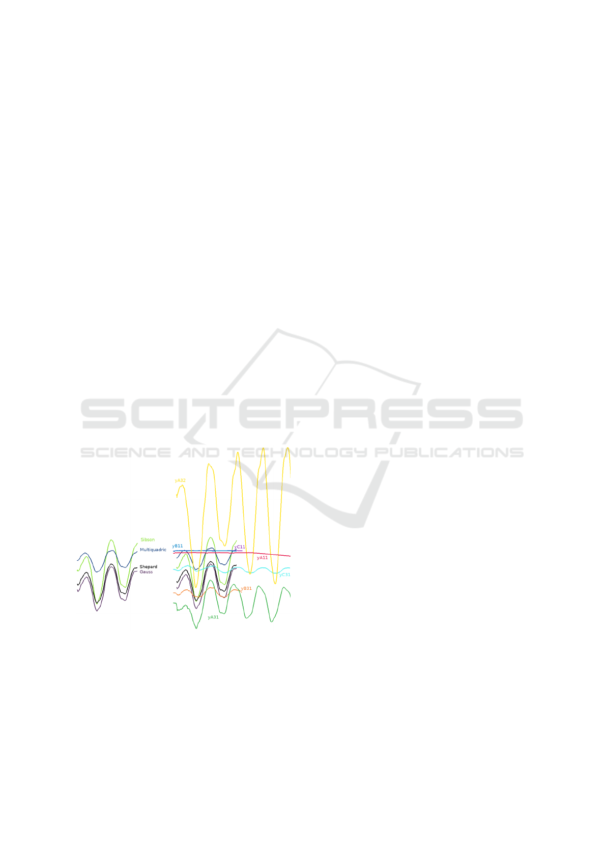
Figure 1: Comparison of interpolation methods for predic-

tion of new run (height 1 km, radius of 240 m, angle of 50

◦

)

using all existing runs in the 1D-over-time multi-run plot.

Predicted runs are qualitatively similar (left) and reﬂect the

oscillatory behavior of existing runs (right).

Parameter Space Uncertainty. Since the user may

select any parameter setting for prediction, guidance

to select new parameter settings is desirable. This can

be achieved by displaying the parameter settings of

existing runs in the d-dimensional parameter space to

see their distribution. To further guide the user to po-

tentially interesting parameter settings, we visualize

the uncertainty in the parameter space.

We ﬁrst need to estimate the uncertainties. To do

so, we sample the d-dimensional parameter space us-

ing an equidistant sampling strategy, which leads to a

d-dimensional uncertainty ﬁeld deﬁned over a regu-

lar grid. For each grid point, we compute the uncer-

tainty that is associated with the respective parameter

setting using the uncertainty measures of Section 5.

More precisely, we estimate the predicted simulation

outcome and its uncertainty as in Section 6. As the

uncertainty in Section 6 was computed per time step,

we now average the uncertainty over all time steps

to obtain a single scalar uncertainty value that is as-

sociated with each grid point of the parameter space

sampling.

We propose to visualize the given ﬁeld by interac-

tively choosing an axis-aligned 2D slice through the

parameter space and to perform a color mapping of

the uncertainty values. We refer to this concept as the

uncertainty map. A 2D slice-based approach is desir-

able, as it has no inherent occlusion issues and scales

to dimensionality d beyond three dimensions. The

resolution of the slice can be chosen by the user and

trilinear interpolation is used to interpolate the uncer-

tainty at any point on the slice.

We implemented our entire system within Voreen

(Meyer-Spradow et al., 2009), a rapid application de-

velopment framework for interactive volume visual-

ization. All prediction and uncertainty visualization

methods have been incorporated into the framework

for a smooth user experience. Figure 6 shows the

slice-based visualization of an uncertainty map.

7 APPLICATION SCENARIO

We apply our approach to the simulation ensemble of

deep water impact by asteroids that hit the Earth’s sur-

face in the ocean (Patchett and Gisler, 2017), where

each simulation run is represented by time-varying

volumetric multi-ﬁeld data with 300

spatial grid

points and varying number of adaptive time steps (be-

tween 162 and 487). The ensemble data is made avail-

able through the IEEE SciVis Contest 2018, unfortu-

nately only comprising seven runs with three scalar

ﬁelds (pressure, temperature, and volume fraction of

water). The parameter space consists of three param-

eters: the height of the airburst (zero in case of no

airburst), the size of the asteroid, and the angle of en-

try. Table 1 lists the seven runs and their parameter

IVAPP 2019 - 10th International Conference on Information Visualization Theory and Applications

220

settings. We used multiﬁeld similarities (Fofonov and

Linsen, 2018b) such that all ﬁelds are considered and

we did not have to choose representative isovalues.

Table 1: Parameter settings of Deep Water Impact simula-

tion ensemble.

Run Radius Angle Height

yA11 100m 45

◦

0km

yA31 250m 45

◦

0km

yA32 250m 60

◦

0km

yB11 100m 45

◦

5km

yB31 250m 45

◦

5km

yC11 100m 45

◦

10km

yC31 250m 45

◦

10km

Prediction. To document that the interpolation-based

prediction is producing suitable results, we ﬁrst made

a simple test that makes prediction considering only

two simulation runs, yA31 and yC31. The two runs

have the same parameter setting for asteroid radius

and incoming angle, but differ in the height of the air-

burst, where yA31 had no airburst and yC31 had an

airburst at height 10km. We predicted runs that were

in between by sampling the airburst height equidis-

tantly with step size 2km. Figure 3 shows the predic-

tion when using inverse-distance-based interpolation

and 1D multi-run plots over time. For all our exam-

ples, the predicted line stops as soon as one of the ex-

isting runs used for interpolation has no further data.

The results indeed deliver the expected and desired re-

sults, as the predicted runs smoothly vary between the

existing runs when varying the simulation parameter.

Next, we wanted to investigate the behavior of the

prediction when using different interpolation methods

on all existing runs within the 3D parameter space.

The parameter settings for the predicted run were an

airburst at height 1 km, an asteroid radius of 240 m,

and an entry angle of 50

◦

. The 1D-over-time multi-

run plots in Figure 1(left) show that all predictions

are qualitatively similar by exhibiting an oscillatory

behavior, but location and amplitude of the curves

vary. Inverse-distance-based and Gaussian radial-

basis-function interpolation produce the most similar

results. When comparing the different prediction re-

sults to the existing runs in Figure 1(right), one can

observe that the oscillatory behavior of the existing

runs is preserved.

To test the quality of our prediction in compar-

ison to running an actual simulation, we performed

a leave-one-out test. Thus, we removed simulation

run yC11 from the ensemble, then tried to predict run

yC11, and compared the predicted to the simulated

outcome. Note that the prediction is actually per-

forming an extrapolation here. Still, all interpolation

methods are applicable except for the natural neigh-

bor interpolation, where our implementation required

the predicted parameter setting to lie inside the con-

vex hull of the existing parameter settings. Figure 2

shows the predicted results in comparison to the sim-

ulated result (labeled as yC11) for the water fraction

ﬁeld. The left side of the ﬁgure shows a 2D multi-run

plot, where time in encoded by the brightness of the

colors. We observe that the multiquadric radial-basis-

function interpolation is producing results that are far

from yC11, while Gaussian radial-basis-function in-

terpolation and Shepard inverse-distance-based inter-

polation are very close. Since the variation of those

runs is small when compared to other runs, we inter-

actively select only the predicted runs and run yC11

and visualize them in a 1D-over-time multi-run plot

on the right side of the ﬁgure. We observe that the

Gaussian radial-basis-function interpolation produces

a prediction that is very close to the simulated run,

as the curves are almost coinciding. Similar obser-

vations can be made for the other ﬁelds such that we

can conclude that the Gaussian radial-basis-function

prediction is in surprisingly high agreement with the

actual simulated run.

Prediction Uncertainty. To illustrate the predic-

tion uncertainty visualization within the multi-run

plots, we predict the pressure ﬁeld of run yB31 using

inverse-distance-based interpolation. Figure 4 shows

the bands with respect to various uncertainties. The

distance-based uncertainty shall be interpreted quali-

tatively only, i.e., it is more meaningful for comparing

different predictions as in the uncertainty map (see be-

low). The interpolation-based uncertainty visualiza-

tion illustrates that there is some variation in the pre-

diction when using different methods, which matches

our observations from above. Still, the simulated run

is not completely within the band such that we can

conclude that the different interpolation methods gen-

erally do not predict the outcome as well as for run

yC11 above. The diversity-based uncertainty shows

up to be larger. This is caused by the fact that we

only have six existing runs (when leaving out yB31),

whose parameter settings have similar distances in pa-

rameter space. Since the existing runs are quite di-

verse in the simulation outcome, the diversity-based

uncertainty is high throughout the prediction. Thus,

the complete uncertainty obtained by compositing the

three uncertainty aspects is also pretty high. The re-

spective band (partially cropped) embeds run yB31.

Parameter Space Uncertainty. The uncertainty

within the 3D parameter space is visualized using the

slice-based views shown in Figure 6, where the X-axis

represents the airburst height (0km-10km), the Y -axis

represents the asteroid’s radius (100m-250m), and the

Uncertainty-aware Prediction in Spatio-temporal Simulation Ensemble Visualizations

221

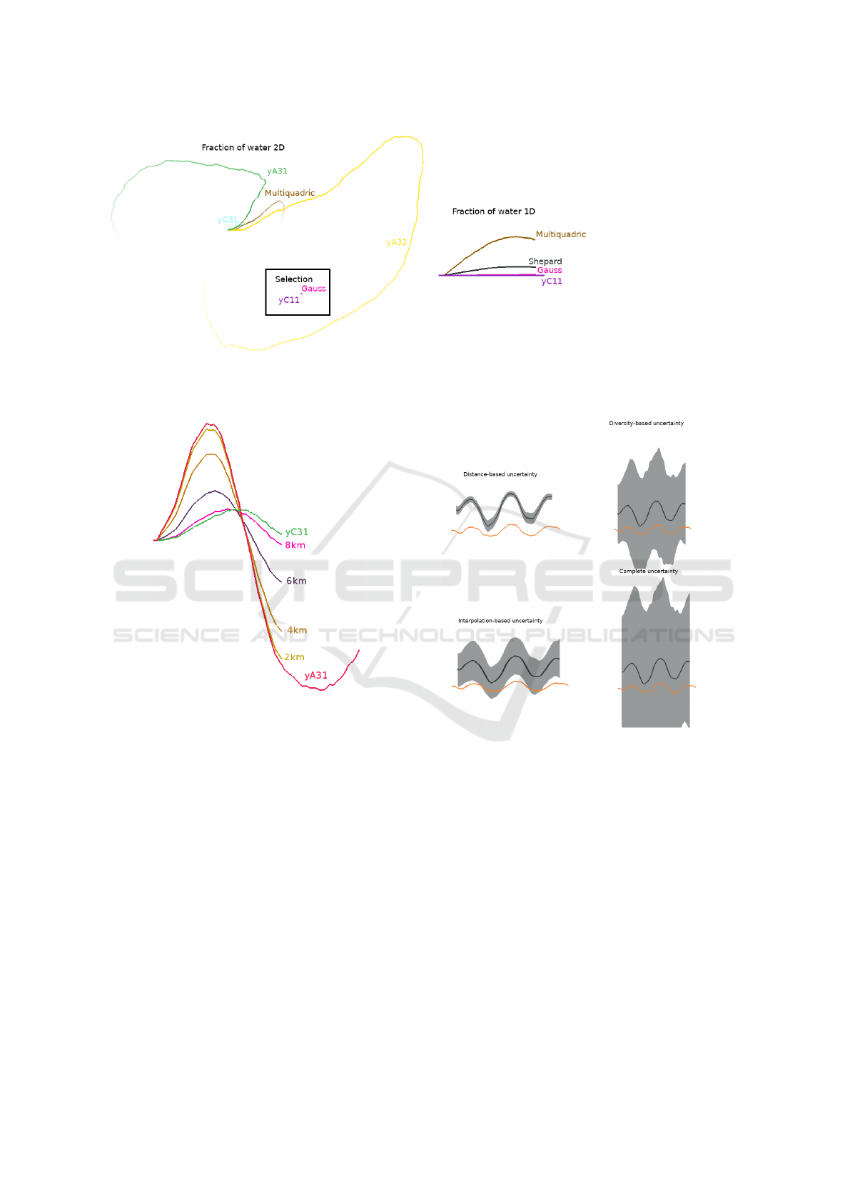
Figure 2: Interpolation results for the fraction of water using different methods for the parameters of the run yC11. In the left

image, the time is colour coded. In the box with the black boundary, a selection of only the interpolation result produced with

Gaussian kernels and the original run can be seen. It is located in the point where all the other runs also start.

Figure 3: Prediction by interpolating between two runs

(yA31 and yC31) delivers a smooth transition between the

runs in the 1D-over-time multi-run plot. Inverse-distance-

based interpolation with exponent 2 was chosen.

Z-axis represents the entry angle (45

◦

-60

◦

). The 3D

uncertainty ﬁeld within the parameters’ range was es-

timated using the introduced uncertainty measures at

samples.

Figure 6a shows the distance-based uncertainty. It

can be observed how the uncertainty increases with

increasing distance from the existing runs’ parameter

settings depicted by the black dots (two black dots are

occluded by the plane).

Figure 6b shows a different distribution of uncer-

tainties when considering diversity. The largest un-

certainty can be observed around the point with height

0 km, angle 60

◦

, and radius 175 m. By construction,

uncertainties are low close to parameter settings of ex-

isting runs, which can be observed. However, it can

also be observed that uncertainties are quite high close

Figure 4: Uncertainty visualization in 1D-over-time multi-

run plots for predicting the pressure ﬁeld of run yB31 (or-

ange). The prediction (black) is obtained using Shepard’s

inverse-distance-based interpolation.

to run yA32 (the only one with angle 60

◦

) in the up-

per left corner of the slice. This was to be expected,

as the simulation outcome of this run is quite different

from the others.

This effect is even stronger for the interpolation-

based uncertainty visualization in Figure 6c, where

the highest uncertainties are computed in the larger

vicinity of run yA32. The large differences between

run yA32 and other runs lead to strongly different in-

terpolation results. It is also interesting that the un-

certainties for height 5km are less than for height 0km

despite the fact that 3 runs with height 0km exist and

only 2 runs with height 5km. Thus, the interpolation-

based uncertainty is not mainly inﬂuenced by dis-

IVAPP 2019 - 10th International Conference on Information Visualization Theory and Applications

222

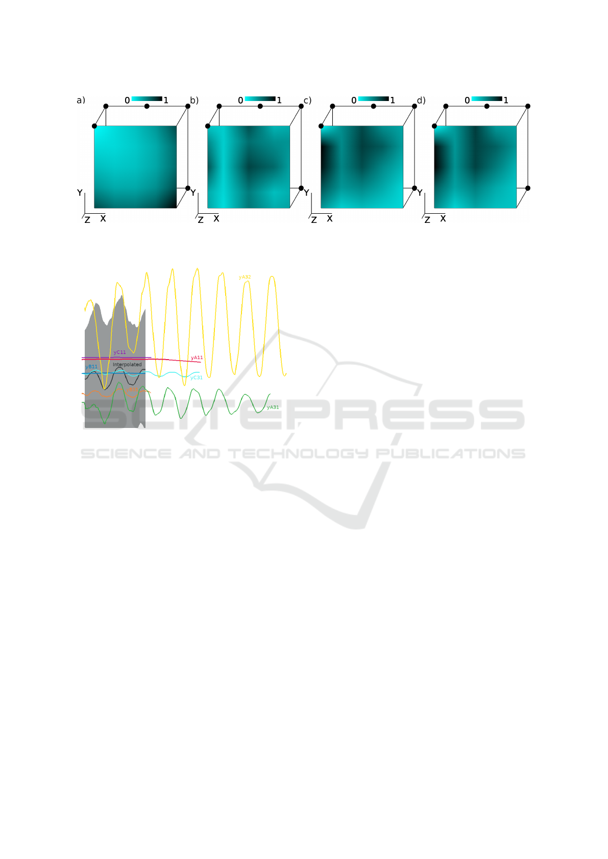
Figure 6: Visualization uncertainty in parameter space (X: airburst height, Y: asteroid radius, Z: entry angle) using 2D slices

(Z=60

◦

) through the uncertainty maps: a) Distance-based uncertainty. b) Diversity-based uncertainty. c) Interpolation-based

uncertainty. d) Composited uncertainty.

Figure 5: Composited uncertainty visualization in 1D-over-

time multi-run plots for predicting the pressure ﬁeld of run

yB31 (orange). The prediction (black) is obtained using

Shepard’s inverse-distance-based interpolation.

tances.

The composited uncertainty map is shown in Fig-

ure 6d. It combines the different aspects of the un-

certainty measures. We can conclude that the desired

properties are achieved: Uncertainty vanishes at the

parameter settings of existing points, it increases with

increasing distance in their vicinity, and the uncer-

tainty ﬁeld is smooth.

8 DISCUSSION AND

CONCLUSION

We proposed a method for predicting simulation out-

comes by interpolating feature vectors and for esti-

mating and visualizing the uncertainties in the pre-

diction. The uncertainty map helps to identify good

choices for further simulation runs in the sense of

computational steering. In our experiments, the Gaus-

sian radial-basis-function interpolation produced the

best prediction results. However, one should also

look into the nature of the analyzed physical simu-

lations. The simulation outcome shall vary smoothly

with changing parameter settings. In future work, it

would be interesting to apply the approach to larger

data sets. Computation times may then be a challenge

again. Generating the uncertainty map over a high-

resolution sample grid (especially when also parame-

ter space is of higher dimension) would also require

quite some computation time. Still, the computation

times are expected to be several order of magnitudes

lower than running the actual simulations. One way of

speeding the computations up would be the usage of

an adaptive time stepping scheme for prediction and

uncertainty estimation.

ACKNOWLEDGMENTS

This work was partially supported by the Deutsche

Forschungsgemeinschaft (DFG) under contract LI

1530/21-1.

REFERENCES

Berger, W., Piringer, H., Filzmoser, P., and Gr

oller, E.

(2011). Uncertainty-aware exploration of continuous

parameter spaces using multivariate prediction. Com-

put Graphics Forum, 30(3):911–920.

Buhmann, M. D. (2000). Radial basis functions. Acta Nu-

merica, 9:1–38.

Cueto, E., Sukumar, N., Calvo, B., Mart

ınez, M., Cego-

nino, J., and Doblar

e, M. (2003). Overview and re-

cent advances in natural neighbour galerkin methods.

Archives of computational methods in engineering,

10(4):307–384.

Fofonov, A. and Linsen, L. (2018a). Multivisa: Visual anal-

ysis of multi-run physical simulation data using inter-

active aggregated plots. In Proceedings of the 13th

International Joint Conference on Computer Vision,

Uncertainty-aware Prediction in Spatio-temporal Simulation Ensemble Visualizations

223

Imaging and Computer Graphics Theory and Appli-

cations (VISIGRAPP 2018) - Volume 3: IVAPP, Fun-

chal, Madeira, Portugal, January 27-29, 2018., pages

62–73.

Fofonov, A. and Linsen, L. (2018b). Projected ﬁeld similar-

ity for comparative visualization of multi-run multi-

ﬁeld time-varying spatial data. Computer Graphics

Forum.

Fofonov, A., Molchanov, V., and Linsen, L. (2016). Visual

analysis of multi-run spatio-temporal simulations us-

ing isocontour similarity for projected views. IEEE

Trans. Visual Comput. Graphics, 22(8):2037–2050.

Griethe, H. and Schumann, H. (2006). The visualization of

uncertain data: Methods and problems. Proceedings

of International Conference on Perspectives in Busi-

ness Informatics Research, 2006.

Liu, S., Maljovec, D., Wang, B., Bremer, P. T., and Pas-

cucci, V. (2017). Visualizing high-dimensional data:

Advances in the past decade. IEEE Trans. Visual

Comput. Graphics, 23(3):1249–1268.

Matkovic, K., Gracanin, D., Jelovic, M., and Hauser, H.

(2008). Interactive visual steering - rapid visual proto-

typing of a common rail injection system. IEEE Trans.

Visual Comput. Graphics, 14(6):1699–1706.

Meyer-Spradow, J., Ropinski, T., Mensmann, J., and Hin-

richs, K. (2009). Voreen: A rapid-prototyping envi-

ronment for ray-casting-based volume visualizations.

IEEE Computer Graphics and Applications, 29(6):6–

13.

Mirzargar, M., Whitaker, R. T., and Kirby, R. M. (2014).

Curve boxplot: Generalization of boxplot for ensem-

bles of curves. IEEE Transactions on Visualization &

Computer Graphics, 20(12):2654–2663.

Pang, A. T., Wittenbrink, C. M., and Lodha, S. K. (1997).

Approaches to uncertainty visualization. The Visual

Computer, 13(8):370–390.

Park, S. W., Linsen, L., Kreylos, O., Owens, J. D., and

Hamann, B. (2006). Discrete sibson interpolation.

IEEE Transactions on visualization and computer

graphics, 12(2):243–253.

Patchett, J. M. and Gisler, G. R. (2017). Deep water impact

ensemble data set. http://sciviscontest2018.org/.

Phadke, M. N., Pinto, L., Alabi, O., Harter, J., Taylor, R. M.,

Wu, X., Petersen, H., Bass, S. A., and Healey, C. G.

(2012). Exploring ensemble visualization. Proc.SPIE,

8294:8294 – 8294 – 12.

Potter, K., Rosen, P., and Johnson, C. R. (2012). From quan-

tiﬁcation to visualization: A taxonomy of uncertainty

visualization approaches. In Dienstfrey, A. M. and

Boisvert, R. F., editors, Uncertainty Quantiﬁcation in

Scientiﬁc Computing, pages 226–249, Berlin, Heidel-

berg. Springer Berlin Heidelberg.

Potter, K., Wilson, A., Bremer, P. T., Williams, D., Dou-

triaux, C., Pascucci, V., and Johnson, C. R. (2009).

Ensemble-vis: A framework for the statistical visual-

ization of ensemble data. In 2009 IEEE International

Conference on Data Mining Workshops, pages 233–

240.

Potter, K. C., Brunhart-Lupo, N. J., Bush, B. W., Gruchalla,

K. M., Bugbee, B., and Krishnan, V. K. (2017).

Coupling visualization, simulation, and deep learn-

ing for ensemble steering of complex energy models:

Preprint.

Rhodes, P. J., Laramee, R. S., Bergeron, R. D., Sparr, T. M.,

et al. (2003). Uncertainty visualization methods in

isosurface rendering. In Eurographics, volume 2003,

pages 83–88.

Sanyal, J., Zhang, S., Dyer, J., Mercer, A., Amburn, P.,

and Moorhead, R. (2010). Noodles: A tool for vi-

sualization of numerical weather model ensemble un-

certainty. IEEE Trans. Visual Comput. Graphics,

16(6):1421–1430.

Sedlmair, M., Heinzl, C., Bruckner, S., Piringer, H., and

oller, T. (2014). Visual parameter space analysis:

A conceptual framework. IEEE Trans Visual Comput

Graphics, 20(12):2161–2170.

Shepard, D. (1968). A two-dimensional interpolation func-

tion for irregularly-spaced data. In Proceedings of

the 1968 23rd ACM National Conference, ACM ’68,

pages 517–524, New York, NY, USA. ACM.

Sibson, R. (1980). A vector identity for the dirichlet tessel-

lation. Mathematical Proceedings of the Cambridge

Philosophical Society, 87(1):151–155.

Splechtna, R., Matkovi

c, K., Gra

canin, D., Jelovi

c, M., and

Hauser, H. (2015). Interactive visual steering of hi-

erarchical simulation ensembles. In 2015 IEEE Con-

ference on Visual Analytics Science and Technology

(VAST), pages 89–96.

Sun, Y. and Genton, M. G. (2011). Functional boxplots.

Journal of Computational and Graphical Statistics,

20(2):316–334.

Waser, J., Fuchs, R., Ribicic, H., Schindler, B., Bloschl,

G., and Groller, E. (2010). World lines. IEEE Trans.

Visual Comput. Graphics, 16(6):1458–1467.

Wickelmaier, F. (2003). An introduction to mds. Sound

Quality Research Unit, Aalborg University, Denmark,

46(5).

Xie, J., Sauer, F., and Ma, K.-L. (2015). Fast uncertainty-

driven large-scale volume feature extraction on desk-

top pcs. In Large Data Analysis and Visualization

(LDAV), 2015 IEEE 5th Symposium on, pages 17–24.

IEEE.

IVAPP 2019 - 10th International Conference on Information Visualization Theory and Applications

224