
Dual SVM Training on a Budget
Sahar Qaadan, Merlin Sch¨uler and Tobias Glasmachers
Department of Neural Computing, Ruhr University Bochum, 44801, Bochum, Germany
Keywords:
Dual Subspace Algorithm, Kernel SVM, Budget Maintenance, Merging Method.
Abstract:
We present a dual subspace ascent algorithm for support vector machine training that respects a budget con-
straint limiting the number of support vectors. Budget methods are effective for reducing the training time
of kernel SVM while retaining high accuracy. To date, budget training is available only for primal (SGD-
based) solvers. Dual subspace ascent methods like sequential minimal optimization are attractive for their
good adaptation to the problem structure, their fast convergence rate, and their practical speed. By incorpo-
rating a budget constraint into a dual algorithm, our method enjoys the best of both worlds. We demonstrate
considerable speed-ups over primal budget training methods.
1 INTRODUCTION
Support Vector Machines (SVMs) introduced by
(Cortes and Vapnik, 1995) are popular machine learn-
ing methods, in particular for binary classification.
They are supported by learning-theoreticalguarantees
(Mohri et al., 2012), and they exhibit excellent gener-
alization performance in many applications in science
and technology (Son et al., 2010; Shigeo, 2005; Byun
and Lee, 2002; Quinlan et al., 2003).They belong to
the family of kernel methods, applying a linear algo-
rithm in a feature space defined implicitly by a kernel
function.
Training an SVM corresponds to solving a large-
scale optimization problem, which can be cast
into a quadratic program (QP). The primal prob-
lem can be solved directly with stochastic gradi-
ent descent (SGD) and accelerated variants (Shalev-
Shwartz et al., 2007; Glasmachers, 2016), while the
dual QP is solved with subspace ascent, see (Bottou
and Lin, 2006) and references therein.
The computational complexity of each stochastic
gradient or coordinate step is governed by the cost of
evaluating the model of a training point. This cost is
proportional to the number of support vectors, which
grows at a linear rate with the data set size (Steinwart,
2003). This limits the applicability of kernel meth-
ods to large-scale data. Efficient algorithms are avail-
able for linear SVMs (SVMs without kernel) (Shalev-
Shwartz et al., 2007; Fan et al., 2008). Parallelization
can yield considerable speed-ups (Wen et al., 2017),
but only by a constant factor. For non-linear (kernel-
ized) SVMs there exists a wide variety of approaches
for approximate SVM training, many of which aim to
leverage fast linear solvers by approximating the fea-
ture space representation of the data. The approxima-
tion can either be fixed (e.g., random Fourier features)
(Lu et al., 2016; Le et al., 2016; Nguyen et al., 2017)
or data-dependent(e.g., Nystr¨om sampling) (Lu et al.,
2016; Rahimi and Recht, 2008; Yang et al., 2012; Ca-
landriello et al., 2017).
Several online algorithms fix the number of SVs to
pre-specified value B ≪ n, the budget, and update the
model in a greedy manner. This way they limit the
iteration complexity. The Stoptron (Orabona et al.,
2009) is a simple algorithm that terminates when the
number of SVs reaches the budget B. The Forgetron
algorithm (Dekel et al., 2008) removes the oldest SV
when the number of SVs exceeds the budget. Un-
der some mild assumptions, convergence of the al-
gorithm has been proven. The Projectron (Orabona
et al., 2009) projects the SV to be removed on the
remaining SVs to minimize the weight degradation.
While the latter outperforms the Forgetron, it requires
O(B)
3
time to compute the projection. Recently, (Lu
et al., 2018) have implemented an efficient stochas-
tic sampling strategy based on turning the incoming
training example into a new support vector with prob-
ability proportional to the loss suffered by the exam-
ple. This method aims to convert the online classifiers
for batch classification purposes.
The above approach can be based on stochastic
gradient descent and combined with more elaborate
budget maintenance techniques (Dekel and Singer,
2007). In particular with the popular budget main-
tenance heuristic of merging support vectors (Wang
94
Qaadan, S., Schüler, M. and Glasmachers, T.
Dual SVM Training on a Budget.
DOI: 10.5220/0007346400940106
In Proceedings of the 8th International Conference on Pattern Recognition Applications and Methods (ICPRAM 2019), pages 94-106
ISBN: 978-989-758-351-3
Copyright
c
2019 by SCITEPRESS – Science and Technology Publications, Lda. All rights reserved

et al., 2012), it goes beyond the above techniques by
adapting the feature space representation during train-
ing. The technique is known as budgeted stochastic
gradient descent (BSGD).
In this context we design the first dual SVM train-
ing algorithm with a budget constraint. The solver
aims at the efficiency of dual subspace ascent as used
in LIBSVM, ThunderSVM, and also in LIBLINEAR
(Chang and Lin, 2011; Fan et al., 2008; Wen et al.,
2017), while applying merging-based budget mainte-
nance as in the BSGD method (Wang et al., 2012).
The combination is far from straight-forward, since
continually changing the feature representation also
implies changing the dual QP, which hence becomes
a moving target. Nevertheless, we provide guarantees
roughly comparable to those available for BSGD.
In a nutshell, our contributions are:
• We present the first dual decomposition algorithm
operating on a budget,
• we analyze its convergence behavior,
• and we establish empirically its superiority to pri-
mal BSGD.
The structure of the paper is as follows: In the next
section we introduce SVMs and existing primal and
dual solvers, including BSGD. Then we present our
novel dual budget algorithm and analyze its asymp-
totic behavior. We compare our method empirically
to BSGD and validate our theoretical analysis. We
close with our conclusions.
2 SUPPORT VECTOR MACHINE
TRAINING
A Support Vector Machine is a supervised kernel
learning algorithm (Cortes and Vapnik, 1995). Given
labeled training data (x
1
,y
1
),. ..,(x
n
,y
n
) ∈ X ×Y and
a kernel function k : X × X → R over the input space,
the SVM decision function f(x) 7→ hw,φ(x)i (we drop
the bias, c.f. (Steinwart et al., 2011)) is defined as the
optimal solution w
∗
of the (primal) optimization prob-
lem
min
w∈H
P(w) =
λ
2
kwk
2
+
1
n
n
∑
i=1
L
y
i
, f(x
i
)
, (1)
where λ > 0 is a regularization parameter, L is a loss
function (usually convex in w, turning problem (1)
into a convex problem), and φ : X → H is an only im-
plicitly defined feature map into the reproducing ker-
nel Hilbert space H , fulfilling hφ(x),φ(x
′
)i = k(x,x
′
).
The representer theorem allows to restrict the solution
to the form w =
∑
n
i=1
α
i
y
i
φ(x
i
) with coefficient vector
α ∈ R
n
, yielding f(x) =
∑
n
i=1
α
i
y
i
k(x,x
i
). Training
points x
i
with non-zero coefficients α
i
6= 0 are called
support vectors.
We focus on the simplest case of binary classi-
fication with label space Y = {−1, +1}, hinge loss
L(y, f(x)) = max{0,1 − yf(x)}, and classifier x 7→
sign( f(x)), however, noting that other tasks like
multi-class classification and regression can be tack-
led in the exact same framework, with minor changes.
For binary classification, the equivalent dual problem
(Bottou and Lin, 2006) reads
max
α∈[0,C]
n
D(α) =
T
α−
1
2
α
T
Qα, (2)
which is a box-constrained quadratic program (QP),
with
= (1,...,1)
T
and C =
1
λn
. The matrix Q con-
sists of the entries Q
ij
= y
i
y
j
k(x
i
,x
j
).
Kernel SVM Solvers. Dual decomposition solvers
like LIBSVM (Chang and Lin, 2011; Bottou and Lin,
2006) are the method of choice for obtaining a high-
precision non-linear (kernelized) SVM solution. They
work by decomposing the dual problem into a se-
quence of smaller problems of size O(1), and solv-
ing the overall problem in a subspace ascent manner.
For problem (2) this can amount to coordinate ascent
(CA). Keeping track of the dual gradient ∇
α
D(α) =
− Qα allows for the application of elaborate heuris-
tics for deciding which coordinate to optimize next,
based on the violation of the Karush-Kuhn-Tucker
conditions or even taking second order information
into account. Provided that coordinate i is to be op-
timized in the current iteration, the sub-problem re-
stricted to α
i
is a one-dimensional QP, which is solved
optimally by the truncated Newton step
α
i
←
α
i
+
1− Q
i
α
Q
ii
C
0
, (3)
where Q
i
is the i-th row of Q and [x]
C
0
=
max
0,min{C,x}
denotes truncation to the box
constraints. The method enjoys locally linear conver-
gence (Lin, 2001), polynomial worst-case complexity
(List and Simon, 2005), and fast convergence in prac-
tice.
In principle the primal problem (1) can be solved
directly, e.g., with SGD, which is at the core of the
kernelized Pegasos algorithm (Shalev-Shwartz et al.,
2007). Replacing the average loss (empirical risk)
in equation (1) with the loss L(y
i
, f(x
i
)) on a single
training point selected uniformly at random provides
an unbiased estimate. Following its (stochastic) sub-
gradient with learning rate 1/(λt) = (nC)/t in itera-
tion t yields the update
α ← α−
α
t
+ 1
{y
i
f(x
i
)<1}
nC
t
e
i
, (4)
Dual SVM Training on a Budget
95

where e
i
is the i-th unit vector and 1
{E}
is the indicator
function of the event E. Despite fast initial progress,
the procedurecan take a long time to produce accurate
results, since SGD suffers from the non-smooth hinge
loss, resulting in slow convergence.
In both algorithms, the iteration complexity is
governed by the computation of f(x) (or equivalently,
by the update of the dual gradient), which is linear in
the number of non-zero coefficients α
i
. This is a lim-
iting factor when working with large-scale data, since
the number of support vectors is usually linear in the
data set size n (Steinwart, 2003).
Linear SVM Solvers. Specialized solvers for lin-
ear SVMs with X = R
d
and φ chosen as the iden-
tity mapping exploit the fact that the weight vector
w ∈ R
d
can be represented directly. This lowers the
iteration complexity from O(n) to O(d) (or the num-
ber of non-zero features in x
i
), which often results in
significant savings (Joachims, 2006; Shalev-Shwartz
et al., 2007). This works even for dual CA by keep-
ing track of the direct representation w and the (re-
dundant) coefficients α, however, at the price that the
algorithm cannot keep track of the dual gradient any
more, which would be an O(n) operation. Therefore
the LIBLINEAR solver resorts to uniform coordinate
selection (Fan et al., 2008), which amountsto stochas-
tic coordinate ascent (SCA) (Nesterov, 2012).
Linear SVMs shine on application domains like
text mining, with sparse data embedded in high-
dimensional input spaces. In general, for moderate
data dimension d ≪ n, separation of the data with a
linear model is a limiting factor that can result in se-
vere under-fitting.
SVMs on a Budget. Lowering the iteration com-
plexity is also the motivation for introducing an upper
bound or budget B ≪ n on the number of support vec-
tors. The budget B is exposed to the user as a hyper-
parameter of the method. The proceeding amounts to
approximating w with a vector ˜w from the non-trivial
fiber bundle
W
B
=
(
B
∑
j=1
β
j
φ( ˜x
j
)
β
1
,. .., β
B
∈ R ; ˜x
1
,. .., ˜x
B
∈ R
d
)
⊂ H .
Critically, W
B
is in general non-convex, and so are
optimization problems over this set. Each SGD step
(eq. (4)) adds at most one new support vector to the
model. If the number of support vectors exceeds B
after such a step, then the budgeted stochastic gradi-
ent descent (BSGD) method applies a budget mainte-
nance heuristic to remove one support vector. Merg-
ing of two support vectors has proven to be a good
compromise between the induced error and the re-
sulting computational effort (Wang et al., 2012). It
amounts to replacing β
i
φ( ˜x
i
)+β
j
φ( ˜x
j
) (with carefully
chosen indices i and j) with a single term β
′
φ( ˜x
′
),
aiming to minimize the “weight degradation” error
kβ
i
φ( ˜x
i
) + β
j
φ( ˜x
j
) − β
′
φ( ˜x
′
)k
2
. For the widely used
Gaussian kernel k(x, x
′
) = exp(−γkx− x
′
k
2
) the opti-
mal ˜x
′
lies on the line spanned by ˜x
i
and ˜x
j
, and it is a
convex combination if merging is restricted to points
of the same class. The coefficient h of the convex
combination ˜x
′
= (1− h) ˜x
i
+ h˜x
j
is found with golden
section search, and the optimal coefficient β
′
is ob-
tained in closed form. This procedure was defined by
(Wang et al., 2012). We use it throughout the rest of
the paper. For completeness sake, the pseudo-code
of the procedure is found in Algorithm 1. It selects
two points from the model with an O(B) heuristic
that aims to minimize the squared weight degradation.
First the point with the smallest coefficient is selected.
The second point is chosen to minimize the squared
weight degradation when merged with the first. These
two points are then merged, i.e., removed from the
model and replaced with the best single-point approx-
imation. We refer to (Wang et al., 2012) for details on
the efficient calculation of the squared weight degra-
dation, as well as on the golden section search proce-
dure used to obtain the coefficient h.
Algorithm 1: Procedure Budget Maintenance for a
sparse model M.
Input/Output: model M =
(β
i
, ˜x
i
)
i∈I
(β
min
, ˜x
min
) ← argmin
|β|
(β, ˜x) ∈ M
WD
∗
← ∞
for (β, ˜x) ∈ M \ {(β
min
, ˜x
min
)} do
m ← β/(β + β
min
)
κ ← k( ˜x, ˜x
min
)
h ← argmax
mκ
(1−h
′
)
2
+(1−m)κ
h
′2
h
′
∈
[0,1]
β
z
← β
min
· κ
(1−h)
2
+ β· κ
h
2
WD ← β
2
min
+ β
2
− β
2
z
+ 2· β
min
· β· κ
if (WD < WD
∗
) then
WD
∗
← WD
(β
∗
, ˜x
∗
,h
∗
,κ
∗
) ← (β, ˜x,h,κ)
end
end
z ← h
∗
· ˜x
min
+ (1− h
∗
) · ˜x
∗
β
z
← β
min
· (κ
∗
)
(1−h
∗
)
2
+ β
∗
· (κ
∗
)
(h
∗
)
2
M ← M \ {(β
min
, ˜x
min
),(β
∗
, ˜x
∗
)} ∪{(β
z
,z)}
In effect, merging allows BSGD to move support
vectors around in the input space. This is well jus-
tified since restricted to W
B
the representer theorem
does not hold. (Wang et al., 2012) show that asymp-
ICPRAM 2019 - 8th International Conference on Pattern Recognition Applications and Methods
96

totically the performance is governed by the approx-
imation error implied by w
∗
6∈ W
B
(see their Theo-
rem 1).
BSGD aims to achieve the best of two worlds,
namely a reasonable compromise between statistical
and computational demands: fast training is achieved
through a bounded computational cost per iteration,
and the application of a kernel keeps the model suffi-
ciently flexible. This requires that B ≪ n basis func-
tions are sufficient to represent a model ˜w that is suf-
ficiently close to the optimal model w
∗
. This assump-
tion is very reasonable, in particular for large n.
3 DUAL COORDINATE ASCENT
WITH BUDGET CONSTRAINT
In this section we present our novel approximate
SVM training algorithm. At its core it is a dual de-
composition algorithm, modified to respect a budget
constraint. It is designed such that the iteration com-
plexity is limited to O(B) operations, and is hence
independent of the data set size n. Our solver com-
bines components from decomposition methods (Os-
una et al., 1997), dual linear SVM solvers (Fan et al.,
2008), and BSGD (Wang et al., 2012) into a new al-
gorithm. Like BSGD, we aim to achieve the best of
two worlds: a-priori limited iteration complexity with
a budget approach, combined with fast convergence
of a dual decomposition solver. Both aspects speed-
up the training process, and hence allow to scale SVM
training to larger problems.
Introducing a budget into a standard decomposi-
tion algorithm as implemented in LIBSVM (Chang
and Lin, 2011) turns out to be non-trivial. Work-
ing with a budget is rather straightforward on the pri-
mal problem (1). The optimization problem is uncon-
strained, allowing BSGD to replace w represented by
α transparently with ˜w represented by coefficients β
j
and flexible basis points ˜x
j
. This is not possible for
the dual problem (2) with constraints formulated di-
rectly in terms of α.
This difficulty is solved by (Fan et al., 2008) for
the linear SVM training problem by keeping track of
w and α. We follow the same approach, however, in
our case the correspondence between w represented
by α and ˜w represented by β
j
and ˜x
j
is only approx-
imate. This is unavoidable by the very nature of the
problem. Luckily, this does not impose major addi-
tional complications.
Algorithm 2: Budgeted Stochastic Coordinate As-
cent (BSCA) Algorithm.
Input: training data (x
1
,y
1
),. ..,(x
n
,y
n
),
k : X × X → R , C > 0, B ∈ N
α ← 0, M ←
/
0
while not happy do
select index i ∈ {1,. ..,n} uniformly at
random
˜
f(x
i
) =
∑
(β, ˜x)∈M
βk(x
i
, ˜x)
δ =
α
i
+
1− y
i
˜
f(x
i
)
/Q
ii
C
0
− α
i
if δ 6= 0 then
α
i
← α
i
+ δ
M ← M ∪ {(δ,x
i
)}
if |M| > B then
trigger budget maintenance, i.e.,
merge two support vectors
end
end
end
return β
The pseudo-code of our Budgeted Stochastic Co-
ordinate Ascent (BSCA) approach is detailed in algo-
rithm 2. It represents the approximate model ˜w as a
set M containing tuples (β, ˜x).
1
Critically, in line 2
the approximate model ˜w is used to compute
˜
f(x
i
) =
h ˜w,x
i
i, so the complexity of this step is O(B). This is
in contrast to the computation of f(x
i
) = hw,x
i
i, with
effort linear in n. At the target iteration cost of O(B) it
is not possible to keep track of the dual gradient, sim-
ply because it consists of n entries that would need
updating with a dense matrix row Q
i
. Consequently,
and in line with (Fan et al., 2008), we resort to uni-
form variable selection in an SCA scheme, and the
role of the coefficients α is reduced to keeping track
of the constraints.
For the budget maintenance procedure, the same
options are available as in BSGD. It is usually imple-
mented as merging of two support vectors, reducing
a model from size |M| = B+ 1 back to size |M| = B.
It is understood that also the complexity of the budget
maintenance procedure should be bounded by O(B)
operations. Furthermore, for the overall algorithm
to work properly, it is important to maintain the ap-
proximate relation ˜w ≈ w. For reasonable settings of
the budget B, this is achieved by non-trivial budget
maintenance procedures like merging and projection
(Wang et al., 2012).
We leave the stopping criterion for the algorithm
open. A stopping criterion akin to (Fan et al., 2008)
based on thresholding KKT violations is not viable,
1
Note that summing over an empty index set simply
yields zero.
Dual SVM Training on a Budget
97

as shown by the subsequent analysis. We therefore
run the algorithm for a fixed number of iterations (or
epochs), as is common for BSGD.
4 ANALYSIS OF BSCA
BSCA is an approximate dual training scheme.
Therefore two questions of major interest are how
quickly it approaches w
∗
, and how close it gets. To
simplify matters somewhat, we make the assumption
that the matrix Q is strictly positive definite. This
ensures that the optimal coefficient vector α
∗
corre-
sponding to w
∗
is unique. For a given weight vector
w =
∑
n
i=1
α
i
y
i
φ(x
i
), we write α(w) when referring to
the corresponding coefficients, which are also unique.
Let w
(t)
and α
(t)
= α(w
(t)
), t ∈ N, denotethe sequence
of solutions generated by an iterative algorithm, using
the labeled training point (x
i
(t)
,y
i
(t)
) for its update in
iteration t. The indices i
(t)
∈ {1,... ,n} are drawn i.i.d.
from the uniform distribution.
Optimization Progressof BSCA. We start by com-
puting the single-iteration progress.
Lemma 1. The change D(α
(t)
) − D(α
(t−1)
) of the
dual objective function in iteration t operating on the
coordinate index i = i
(t)
∈ {1,..., n} equals
J
α
(t−1)
, i, α
(t)
i
− α
(t−1)
i
:=
Q
ii
2
"
1− Q
i
α
(t−1)
Q
ii
#
2
−
"
α
(t)
i
− α
(t−1)
i
−
1− Q
i
α
(t−1)
Q
ii
#
2
.
Proof. Consider the function s(δ) = D(α
(t−1)
+ δe
i
).
It is quadratic with second derivative −Q
ii
< 0 and
with its maximum at δ
∗
= (1− Q
i
α
(t−1)
)/Q
ii
. Repre-
sented by its second order Taylor series around δ
∗
it
reads s(δ) = s(δ
∗
) −
Q
ii
2
(δ − δ
∗
)
2
. This immediately
yields the result.
The lemma is in line with the optimality of the
update (3). Based thereon we define the relative ap-
proximation error
E(w, ˜w) := 1− max
i∈{1,...,n}
J
α(w), i,
h
α
i
(w) +
1−y
i
h ˜w,φ(x
i
)i
Q
ii
i
C
0
− α
i
(w)
J
α(w), i,
h
α
i
(w) +
1−y
i
hw,φ(x
i
)i
Q
ii
i
C
0
− α
i
(w)
.
(5)
The margin calculation in the numerator is based on
˜w, while it is based on w in the denominator. Hence
E(w, ˜w) captures the effect of using ˜w instead of w
in BSCA. Informally, we interpret it as a dual quan-
tity related to the weight degradation error k ˜w− wk
2
.
Lemma 1 implies that the relative approximationerror
is non-negative, because the optimal step is in the de-
nominator, which upper bounds the fraction by one.
It is continuous (and in fact piecewise linear) in ˜w,
for fixed w. Finally, it fulfills ˜w = w ⇒ E(w, ˜w) = 0.
The following theorem bounds the suboptimality of
BSCA, and it captures the intuition that the relative
approximation error poses a principled limit on the
achievable solution precision.
Theorem 1. The sequence α
(t)
produced by BSCA
fulfills
D(α
∗
) − E
h
D(α
(t)
)
i
≤
D(α
∗
) +
nC
2
2
·
t
∏
τ=1
1−
2κ
1− E(w
(τ−1)
, ˜w
(τ−1)
)
(1+ κ)n
!
,
where κ is the smallest eigenvalue of Q.
Proof. Theorem 5 by (Nesterov, 2012) applied to the
non-budgeted setting ensures linear convergence
E[D(α
∗
) − D(α
(t)
)] ≤
D(α
∗
) +
nC
2
2
·
1−
2κ
(1+ κ)n
t
,
and in fact the proof establishes a linear decay of
the expected suboptimality by the factor 1 −
2κ
(1+κ)n
in each single iteration. With a budget in place, the
improvement is further reduced by the difference be-
tween the actual dual progress (the numerator in eq. 5)
and the progress in the non-budgeted case (the de-
nominator in eq. 5). By construction (see lemma 1
and eq. 5), this additive difference, when written as
a multiplicative factor, amounts to 1− E(w, ˜w) in the
worst case. The worst case is reflected by taking the
maximum over i ∈ {1,.. ., n} in eq. 5.
We conclude from Theorem 1 that the behavior
of BSCA can be divided into an early and a late
phase. For fixed weight degradation, the relative ap-
proximation error is small as long as the progress
is sufficiently large, which is the case in early iter-
ations. Then the algorithm is nearly unaffected by
the budget constraint, and multiplicative progress at
a fixed rate is achieved. Progress gradually decays
when approaching the optimum, which increases the
relative approximation error, until BSCA stalls. In
fact, the theorem does not witness further progress
for E(w, ˜w) ≥ 1. Due to w
∗
6∈ W
B
, the KKT violations
do not decay to zero, and the algorithm approaches a
limit distribution.
2
The precision to which the opti-
mal SVM solution can be approximated is hence lim-
ited by the relative approximation error, or indirectly,
by the weight degradation.
2
BSCA does not converge to a unique point. It does not
become clear from the analysis provided by (Wang et al.,
2012) whether this is also the case for BSGD, or whether
the decaying learning rate allows BSGD to converge to a
local minimum.
ICPRAM 2019 - 8th International Conference on Pattern Recognition Applications and Methods
98

Budget Maintenance Rate. The rate at which bud-
get maintenance is triggered can play a role, in partic-
ular if the procedure consumes a considerable share
of the overall runtime. In the following we highlight
a difference between BSGD and BSCA. For an algo-
rithm A let
p
A
= lim
T→∞
E
1
T
·
n
t ∈ {1,. .. ,T}
y
i
(t)
hw
(t−1)
,φ(x
i
(t)
)i < 1
o
denote the expected fraction of optimization steps in
which the target margin is violated, in the limit t → ∞
(if the limit exists). The following lemma establishes
the fraction for primal SGD (eq. (4)) and dual SCA
(eq. (3)), both without budget.
Lemma 2. Under the conditions (i) α
∗
i
∈ {0,C} ⇒
∂D(α
∗
)
∂α
i
6= 0 and (ii)
∂D(α
(t)
)
∂α
i
t
6= 0 (excluding only a zero-
set of cases) it holds p
SGD
=
1
n
∑
n
i=1
α
∗
i
C
and p
SCA
=
1
n
|{i|0 < α
∗
i
< C}|.
Proof. The lemma considers the non-budgeted case,
therefore the training problem is convex. Then the
condition
∑
∞
t=1
1
t
= ∞ for the learning rates ensures
convergence α
(t)
→ α
∗
with SGD. This can happen
only if the subtraction of α
(t−1)
i
and the addition of
nC with learning rate
1
t
cancel out in the update equa-
tion (4) in the limit t → ∞, in expectation. Formally
speaking, we obtain
lim
T→∞
E
"
1
T
T
∑
t=1
1
{
i
(t)
=i
}
1
{
y
i
(t)
hw
(t−1)
,φ(x
i
(t)
)i<1
}
nC− α
(t−1)
i
#
= 0 ∀i ∈ {1,.. ., n},
and hence lim
T→∞
E
h
1
T
∑
T
t=1
1
{
i
(t)
=i
}
1
{
y
i
(t)
hw
(t−1)
,φ(x
i
(t)
)i<1
}
i
=
α
∗
i
nC
. Summation over i completesthe proof of the result
for SGD.
In the dual algorithm, with condition (i) and the
same argument as in (Lin, 2001) there exists an it-
eration t
0
so that for t > t
0
all variables fulfilling
α
∗
i
∈ {0,C} remain fixed: α
(t)
i
= α
(t
0
)
i
, while all other
variables remain free: 0 < α
(t)
i
< C. Assumption
(ii) ensures that all steps on free variables are non-
zero and hence contribute 1/n to p
SCA
in expectation,
which yields p
SCA
=
1
n
|{i|0 < α
∗
i
< C}|.
A point (x
i
(t)
,y
i
(t)
) that violates the target margin
of one is added as a new support vector in BSGD
as well as in BSCA. After the first B such steps, all
further additions trigger budget maintenance. Hence
Lemma 2 gives an asymptotic indication of the num-
ber of budget maintenance events, provided ˜w ≈ w,
i.e., if the budget is not too small. The different rates
for primal and dual algorithm underline the quite dif-
ferent optimization behavior of the two algorithms:
while (B)SGD keeps making non-trivial steps on all
training points corresponding to α
∗
i
> 0 (support vec-
tors w.r.t. w
∗
), after a while the dual algorithm oper-
ates only on the free variables 0 < α
∗
i
< C.
5 EXPERIMENTS
In this section we compare our dual BSCA algorithm
on the binary classification problems ADULT, COD-
RNA, COVERTYPE, IJCNN, and SUSY, covering a
range of different sizes. Moreover, we run BSCA
on a smaller budget. The regularization parameter
C =
1
n·λ
and the kernel parameter γ were tuned with
grid search and cross-validation, see table 1. The C++
implementation of our algorithm is published on the
third author website.
Table 1: Data sets used in this study, hyperparameter set-
tings, test accuracy, number of support vectors, and training
time of the full SVM model (using LIBSVM).
data set size features C γ accuracy #SVs training time
SUSY 4,500,000 18 2
5
2
−7
80.02% 2,052,555 504h25m38s
COVTYPE 581,012 54 2
7
2
−3
75.88% 187,626 10h5m7s
COD-RNA 59,535 8 2
5
2
−3
96.33% 9,120 53.951s
IJCNN 49,990 22 2
5
2
1
98.77% 2,477 46.914s
ADULT 32,561 123 2
5
2
−7
84.82% 11,399 97.152s
Data Sets and Hyperparameters. The test prob-
lems were selected according to the following criteria,
which taken together imply that applying the budget
method is a reasonable choice:
• The feature dimension is not too large. Therefore
a linear SVM performs rather poorly compared to
a kernel machine.
• The problem size is not too small. The range of
sizes spans more than two orders of magnitude.
The hyperparameters C and γ were log
2
encoded and
tuned on an integer grid with cross-validation using
LIBSVM, i.e., aiming for the best possible perfor-
mance of the non-budgeted machine. The budget was
set to B = 500 in all experiments, unless stated other-
wise. This value turns out to offer a reasonable com-
promise between speed and accuracy on all problems
under study.
5.1 Primal vs. Dual Solver
The first step is to compare dual BSCA to its closest
sibling, the primal BSGD method. Both algorithms
maintain the budget by means of merging of pairs of
support vectors.
Optimization Performance. BSCA and BSGD are
optimization algorithms. Hence it is natural to com-
pare them in terms of primal and dual objective func-
Dual SVM Training on a Budget
99
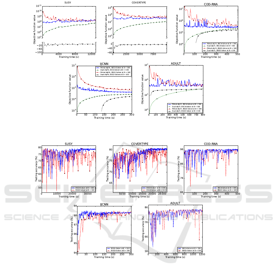
Figure 1: Primal and dual objective function curves of BSGD and BSCA solvers with a budget of B = 500. We use a mixed
linear and logarithmic scale where the dual objective stays negative, which happens for BSGD on two problems.
Figure 2: Test accuracy for the primal and dual solvers at a budget of B = 500 over training time.
tion, see equations (1) and (2). Since the solvers opti-
mize different functions, we monitor both. However,
we consider the primal as being of primary interest
since its minimization is the goal of SVM training,
by definition. Convergence plots are displayed in fig-
ure 1. Overall, the dual BSCA solver clearly outper-
forms the primal BSGD method across all problems.
While the dual objective function values are found
to be smooth and monotonic in all cases, this is not
the case for the primal. BSCA generally oscillates
less and stabilizes faster (with the exception of the
ADULT problem), while BSGD remains somewhat
unstable and is hence at risk of delivering low-quality
solutions for a much longer time when it happens to
stop at one of the peaks.
Learning Performance. Figure 2 shows the corre-
sponding evolution of the test error. In our experi-
ment, all budgeted models reach an accuracy that is
nearly indistinguishable from the exact SVM solu-
tion. The accuracy converges significantly faster for
the dual solver. For the primal solver we observe a
long series of peaks corresponding to significantly re-
duced performance. This observation is in line with
the observed optimization behavior. The effect is par-
ticularly pronounced for the largest data sets SUSY
and COVERTYPE. Moreover, we conduct extensive
experiments to check if the learning performance re-
sults vary in different runs depending upon the order
of data-point considered in the algorithm 1. There-
fore, a variance plot for each data set is shown in fig-
ICPRAM 2019 - 8th International Conference on Pattern Recognition Applications and Methods
100
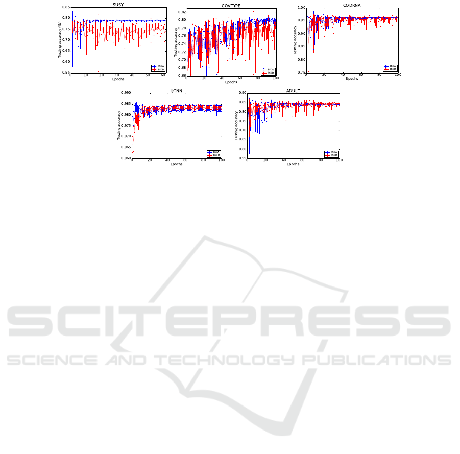
Figure 3: Stability of the test accuracy for the primal and dual solvers at a budget of B = 500. The plots indicate mean and
standard deviation of the test accuracy over 10 independent runs.
ure 3. The plots provide variance curves for the aver-
age over 10 set of experiments.
Convergence Behavior. The next experiment vali-
dates the predictions of Lemma 2 when using a bud-
get. Figure 8 displays the fraction of mergingsteps for
different budget sizes applied to the dual and primal
solvers. We find the predictions of the lemma being
approximately valid also when using a budget. The
figure highlights an interesting difference in the opti-
mization behavior between BSGD and BSCA: while
the former makes non-zero steps on all support vec-
tors (training points with a margin of at most one), the
latter manages to fix the dual variables of margin vio-
lators (training points with a margin strictly less than
one) at the upper bound C.
5.2 Impact of the Budget
In this section we investigate the impact of the budget
and its size on optimization and learning behavior. We
start with an experiment comparing primal and dual
solver without budget. The results are presented in
figure 4. It is apparent that the principal differences
between BSGD and BSCA remain the same when run
without budget constraint, i.e., the most significant
differences stem from the quite different optimization
behavior of stochastic gradient descent and stochas-
tic coordinate ascent. The SGD learning curves are
quite noisy with many downwards peaks. The results
are in line with experiments on linear SVMs by (Fan
et al., 2008; Hsieh et al., 2008). To investigate the
effect of the budget size, Figure 5 provides test ac-
curacy curves for a reduced budget size of B = 200.
For some of the test problems this budget it already
rather small, resulting in sub-optimal learning behav-
ior. Generally speaking, BSCA clearly outperforms
BSGD. However, BSCA fails on the IJCNN data set,
while BSGD fails to deliver high quality solutions
on SUSY and COVERTYPE. Figure 7 aggregates the
data in a different way, comparing the test accuracy
achieved with different budgets on a common time
axis. In this presentation it is easy to read off the
speed-up achievable with a smaller budget. Unsur-
prisingly, BSCA with budget B = 200 is much faster
than the same algorithm with budget B = 500 when
run for the same number of epochs. However, when
it comes to achieving a good test error quickly, the re-
sults are mixed. While the small budget apparently
suffices on COVERTYPE and SUSY, the provided
number of epochs does not suffice to reach good re-
sults on IJCNN, where the solver with B = 500 is sig-
nificantly faster. Figure 6 presents a similar analysis,
but with primal and dual objective function. Overall
it underpins the learning (test accuracy) results, how-
ever, it also reveals a drift effect of the dual solver
in particular for the smaller budget B = 200, with
both objectives rising. This can happen if the weight
degradation becomes large and the gradient computed
based on the budgeted representation does not prop-
erly reflect the dual gradient any more.
5.3 Comparison of BSCA with
Alternative Budgeted Solvers
In this section, we conduct an extensive set of experi-
ments to examine the efficiency of the proposed algo-
rithm in comparison to state-of-the-art approaches for
online kernel learning. To make a fair comparison of
algorithms with different parameters, the RBF kernel
parameter γ and the regularization parameter C were
optimized with 5-fold cross validation on the training
Dual SVM Training on a Budget
101
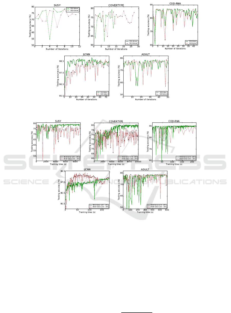
Figure 4: Test accuracy results of solvers based directly on SCA and SGD, without budget. The results are monitored every
300,000 iterations for SUSY and COVERTYPE, and every 10,000 iterations for all other data sets.
Figure 5: Test accuracy results for BSCA and BSGD at a budget of 200.
dataset using LIBSVM. The budget size B and learn-
ing rate η in NOGD and Pegasos and the feature di-
mension D and learning rate η in FOGD are set in-
dividually for different datasets according to the rec-
ommendation of (Lu et al., 2016). For each dataset,
the model is trained in a single pass through the data.
For comparison, we employ 11 state-of-the-art online
kernel learning methods:
• perceptron (Freund and Schapire, 1998),
• online gradient descent (OGD) (Kivinen et al.,
2003),
• randomized budget perceptron (RBP) (Cavallanti
et al., 2007),
• forgetron (Dekel et al., 2008),
• projectron and projectron++ (Orabona et al.,
2009),
• budgeted passive-aggressive simple (BPAS)
(Wang and Vucetic, 2010),
• bounded OGD (BOGD) (Zhao et al., 2012),
• budgeted SGD using merging strategy (BSGD)
(Wang et al., 2012),
• Fourier OGD (FOGD) and Nystrom OGD
(NOGD) (Lu et al., 2016).
Their implementations are published as a part of the
LIBSVM
3
and LSOKL5 toolboxes.
4
The results are
summarized in Table 2.
Our first observation is that the budgeted online
approaches demonstrate their effectiveness with sub-
stantially shorter runtimes than the ones without bud-
3
http://www.csie.ntu.edu.tw/ cjlin/libsvm/
4
http://lsokl.stevenhoi.org
ICPRAM 2019 - 8th International Conference on Pattern Recognition Applications and Methods
102
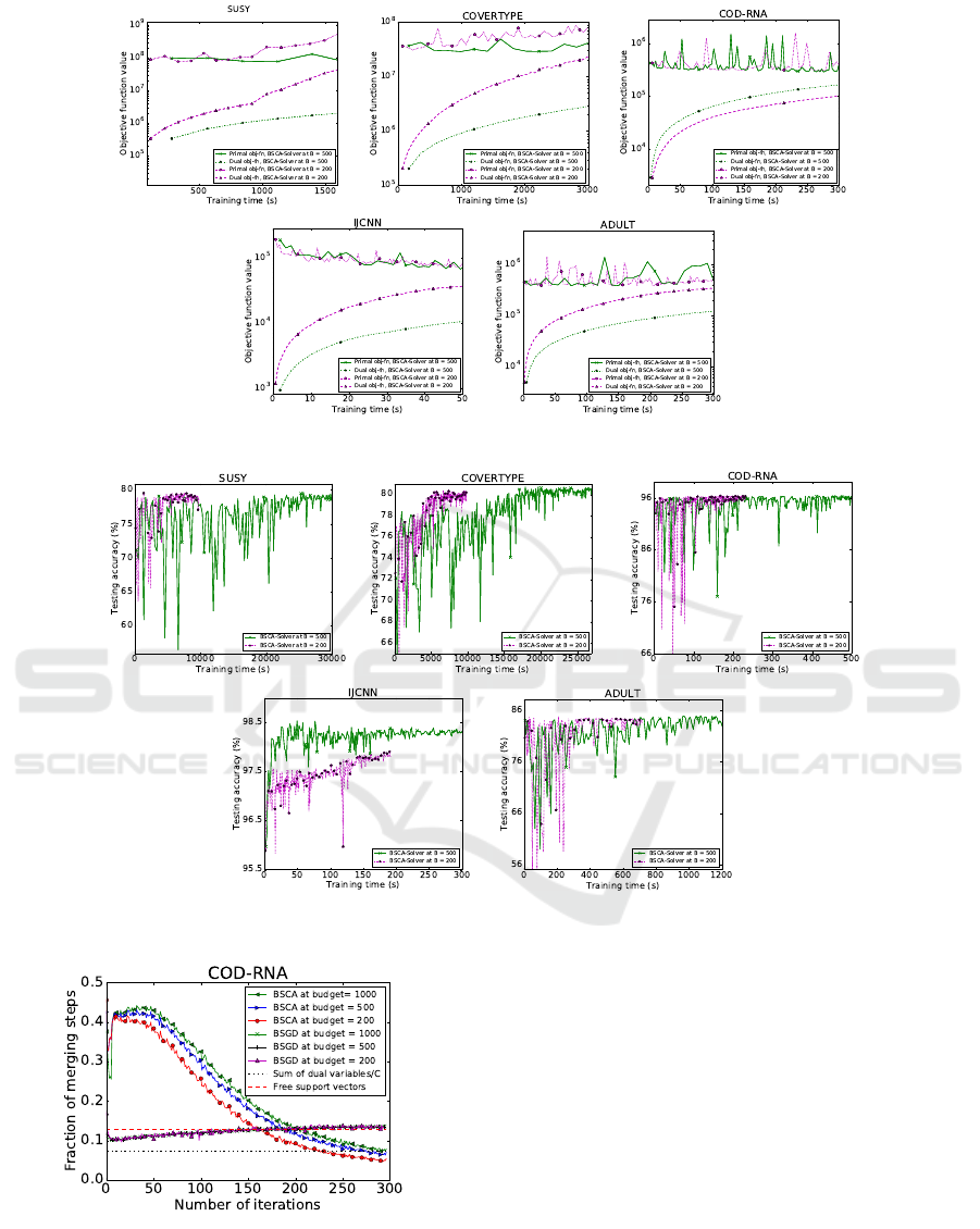
Figure 6: Primal and dual objective function over time for BSCA at budgets B ∈ {200,500}.
Figure 7: Test accuracy over time for BSCA at budgets B ∈ {200,500}.
Figure 8: Fraction of merging steps over a large number of
epochs at budgets B ∈ {200,500,1000}.
gets. More specifically, the execution time of our
proposed model BSCA is much faster than that of
alternative online algorithms and the recent fast al-
gorithms FOGD and NOGD. BCDA is only slightly
slower than the fastest methods which, with the no-
table exception of BPAS, achieve significantly worse
results.
In terms of accuracy, the BSCA method performs
best on IJCNN, and more importantly, it performs
consistently well across all problems. Only the rather
slow online gradient descent approach achieves sim-
ilar performance, but using 8 to 33 times as much
training time, which would allow BSCA to perform
many epochs.
We excluded the SUSY and COVTYPE data sets
from table 2 due to the effort of tuning the param-
eter D for the FOGD method. For example, an ex-
periment using D = 10,000 for FOGD was running
for approximately two hours, achieving a test accu-
Dual SVM Training on a Budget
103

Table 2: Training time (seconds) and testing error (%) comparison between BSCA algorithm and all approaches implemented
by (Lu et al., 2016). The budget size B is fixed to 500 for consistency with the previous experiment. The number of random
features D for FOGD is selected depending on the settings in (Lu et al., 2016), where D is set to 4000, 1600 and 1000 for
ADULT, CODRNA and IJCNN, respectively. For better readability, column-wise best values are highlighted.
ADULT CODRNA IJCNN
Algorithm training time test accuracy training time test accuracy training time test accuracy
Perceptron 53.37 83.35% 60.04 88.12% 25.31 95.75%
OGD 107.02 84.50% 227.25 95.77% 92.90 94.59%
RBP 7.21 76.38% 6.42 95.31% 8.04 91.74%
Forgetron 9.31 83.39% 7.24 92.55% 9.06 92.74%
Projectron 38.80 25.65% 61.79 33.31% 11.98 96.24%
Projectron++ 36.00 82.59% 46.89 71.95% 51.02 96.77%
BPAS 7.69 83.44% 6.76 94.12% 8.86 95.01%
BOGD 8.02 76.38% 6.59 80.77% 8.66 91.01%
BSGD 8.48 80.74% 4.37 89.85% 11.28 96.68%
FOGD 18.00 82.00% 9.17 72.20% 26.13 90.50%
NOGD 37.10 83.15% 38.17 95.62% 40.30 90.50%
BSCA 9.84 83.18% 6.85 95.68% 11.53 97.27%
racy of 49.98% (guessing performance), where BSCA
achieved 77.03%. This observation further validates
the effectiveness and efficiency of our proposed tech-
nique. Thus, we believe that our BSCA algorithm is a
promising technique for building large kernel learning
algorithms for large-scale classification tasks.
5.4 Discussion
Our results do not only indicate that the optimization
behavior of BSGD and BSCA is significantly differ-
ent, they also demonstrate the superiority of the dual
approach for SVM training, in terms of optimization
behavior as well as in terms of test accuracy. We at-
tribute its success to the good fit of coordinate ascent
to the box-constrained dual problem, while the pri-
mal solver effectivelyignores the upper bound (which
is not represented explicitly in the primal problem),
resulting in large oscillations. Importantly, the im-
proved optimization behavior translates directly into
better learning behavior. The introduction of budget
maintenance techniques into the dual solver does not
change this overall picture, and hence yields a viable
route for fast training of kernel machines.
The BSCA method does not only clearly outper-
form the primal BSGD method, but it also performs
very well when compared with alternative fast train-
ing schemes for training kernelized SVMs. The fast
epoch times indicate a low overhead over the margin
computation, which is at the heart of every iterative
method. At the same time our new approach achieves
excellent accuracy.
6 CONCLUDING REMARKS
We have presented the first dual decomposition algo-
rithm for support vector machine training honoring a
budget, i.e., an upper bound on the number of sup-
port vectors. This approximate SVM training algo-
rithm combines fast iterations enabled by the budget
approach with the fast convergence of a dual decom-
position algorithm. Like its primal cousin, it is fun-
damentally limited only by the approximation error
induced by the budget. We demonstrate significant
speed-ups over primal budgeted training, as well as
increased stability. Overall, for training SVMs on a
budget, we can clearly recommend our method as a
plug-in replacement for primal methods. It is rather
straightforward to extend our algorithm to other ker-
nel machines with box-constrained dual problems.
ACKNOWLEDGEMENTS
We acknowledge support by the Deutsche
Forschungsgemeinschaft (DFG) through grant
GL 839/3-1.
REFERENCES
Bottou and Lin, 2006Bottou, L. and Lin, C.-J. (2006). Support
vector machine solvers.
Byun and Lee, 2002Byun, H. and Lee, S.-W. (2002). Applica-
tions of Support Vector Machines for Pattern Recogni-
tion: A Survey, pages 213–236. Springer Berlin Hei-
delberg, Berlin, Heidelberg.
ICPRAM 2019 - 8th International Conference on Pattern Recognition Applications and Methods
104

Calandriello et al., 2017Calandriello, D., Lazaric, A., and
Valko, M. (2017). Efficient second-order online ker-
nel learning with adaptive embedding. In Guyon, I.,
Luxburg, U. V., Bengio, S., Wallach, H., Fergus, R.,
Vishwanathan, S., and Garnett, R., editors, Advances
in Neural Information Processing Systems 30, pages
6140–6150. Curran Associates, Inc.
Cavallanti et al., 2007Cavallanti, G., Cesa-Bianchi, N., and
Gentile, C. (2007). Tracking the best hyperplane
with a simple budget perceptron. Machine Learning,
69(2):143–167.
Chang and Lin, 2011Chang, C.-C. and Lin, C.-J. (2011). LIB-
SVM: A library for support vector machines. ACM
Trans. Intell. Syst. Technol., 2(3).
Cortes and Vapnik, 1995Cortes, C. and Vapnik, V. (1995).
Support-vector networks. Machine learning,
20(3):273–297.
Dekel et al., 2008Dekel, O., Shalev-Shwartz, S., and Singer,
Y. (2008). The forgetron: A kernel-based perceptron
on a budget. SIAM J. Comput., 37(5):1342–1372.
Dekel and Singer, 2007Dekel, O. and Singer, Y. (2007). Sup-
port vector machines on a budget. MIT Press.
Fan et al., 2008Fan, R.-E., Chang, K.-W., Hsieh, C.-J., Wang,
X.-R., and Lin, C.-J. (2008). Liblinear: A library for
large linear classification. J. Mach. Learn. Res., pages
1871–1874.
Freund and Schapire, 1998Freund, Y. and Schapire, R. E.
(1998). Large margin classification using the percep-
tron algorithm. In Proceedings of the Eleventh An-
nual Conference on Computational Learning Theory,
COLT’ 98, New York, NY, USA. ACM.
Glasmachers, 2016Glasmachers, T. (2016). Finite sum accel-
eration vs. adaptive learning rates for the training of
kernel machines on a budget. In NIPS workshop on
Optimization for Machine Learning.
Hsieh et al., 2008Hsieh, C.-J., Chang, K.-W., Lin, C.-J.,
Keerthi, S. S., and Sundararajan, S. (2008). A dual co-
ordinate descent method for large-scale linear SVM.
In Proceedings of the 25th International Conference
on Machine Learning, pages 408–415. ACM.
Joachims, 2006Joachims, T. (2006). Training linear SVMs in
linear time. In Proceedings of the 12th ACM SIGKDD
international conference on Knowledge discovery and
data mining, pages 217–226. ACM.
Kivinen et al., 2003Kivinen, J., Smola, A. J., and Williamson,
R. C. (2003). Online learning with kernels. volume 52,
pages 2165–2176.
Le et al., 2016Le, T., Nguyen, T., Nguyen, V., and Phung, D.
(2016). Dual space gradient descent for online learn-
ing. In Lee, D. D., Sugiyama, M., Luxburg, U. V.,
Guyon, I., and Garnett, R., editors, Advances in Neu-
ral Information Processing Systems 29, pages 4583–
4591. Curran Associates, Inc.
Lin, 2001Lin, C.-J. (2001). On the convergence of the decom-
position method for support vector machines. IEEE
Transactions on Neural Networks, 12(6):1288–1298.
List and Simon, 2005List, N. and Simon, H. U. (2005). Gen-
eral polynomial time decomposition algorithms. In
International Conference on Computational Learning
Theory, pages 308–322. Springer.
Lu et al., 2016Lu, J., Hoi, S. C., Wang, J., Zhao, P., and Liu,
Z.-Y. (2016). Large scale online kernel learning. Jour-
nal of Machine Learning Research, 17(47):1–43.
Lu et al., 2018Lu, J., Sahoo, D., Zhao, P., and Hoi, S.
C. H. (2018). Sparse passive-aggressive learning for
bounded online kernel methods. ACM Trans. Intell.
Syst. Technol., 9(4).
Mohri et al., 2012Mohri, M., Rostamizadeh, A., and Tal-
walkar, A. (2012). Foundations of Machine Learning.
MIT press.
Nesterov, 2012Nesterov, Y. (2012). Efficiency of coordinate
descent methods on huge-scale optimization prob-
lems. SIAM Journal on Optimization, 22(2):341–362.
Nguyen et al., 2017Nguyen, T. D., Le, T., Bui, H., and Phung,
D. (2017). Large-scale online kernel learning with
random feature reparameterization. In Proceedings of
the 26th International Joint Conference on Artificial
Intelligence.
Orabona et al., 2009Orabona, F., Keshet, J., and Caputo, B.
(2009). Bounded kernel-based online learning. J.
Mach. Learn. Res., pages 2643–2666.
Osuna et al., 1997Osuna, E., Freund, R., and Girosi, F. (1997).
An improved training algorithm of support vector ma-
chines. In Neural Networks for Signal Processing VII,
pages 276 – 285.
Quinlan et al., 2003Quinlan, M. J., Chalup, S. K., and Mid-
dleton, R. H. (2003). Techniques for improving vi-
sion and locomotion on the Sony AIBO robot. In In
Proceedings of the 2003 Australasian Conference on
Robotics and Automation.
Rahimi and Recht, 2008Rahimi, A. and Recht, B. (2008).
Random features for large-scale kernel machines. In
Advances in neural information processing systems,
pages 1177–1184.
Shalev-Shwartz et al., 2007Shalev-Shwartz, S., Singer, Y., and
Srebro, N. (2007). Pegasos: Primal estimated sub-
gradient solver for SVM. In Proceedings of the
24th International Conference on Machine Learning,
pages 807–814.
Shigeo, 2005Shigeo, A. (2005). Support Vector Machines for
Pattern Classification (Advances in Pattern Recogni-
tion). Springer-Verlag New York, Inc., Secaucus, NJ,
USA.
Son et al., 2010Son, Y.-J., Kim, H.-G., Kim, E.-H., Choi, S.,
and Lee, S.-K. (2010). Application of support vec-
tor machine for prediction of medication adherence
in heart failure patients. Healthcare Informatics Re-
search, pages 253–259.
Steinwart, 2003Steinwart, I. (2003). Sparseness of support
vector machines. Journal of Machine Learning Re-
search, 4:1071–1105.
Steinwart et al., 2011Steinwart, I., Hush, D., and Scovel, C.
(2011). Training SVMs without offset. Journal of
Machine Learning Research, 12(Jan):141–202.
Wang et al., 2012Wang, Z., Crammer, K., and Vucetic, S.
(2012). Breaking the curse of kernelization: Budgeted
stochastic gradient descent for large-scale SVM train-
ing. J. Mach. Learn. Res., 13(1):3103–3131.
Wang and Vucetic, 2010Wang, Z. and Vucetic, S. (2010). On-
line passive-aggressive algorithms on a budget. In
Dual SVM Training on a Budget
105

Proceedings of the Thirteenth International Confer-
ence on Artificial Intelligence and Statistics, vol-
ume 9, pages 908–915. PMLR.
Wen et al., 2017Wen, Z., Shi, J., He, B., Li, Q., and Chen, J.
(2017). ThunderSVM: A fast SVM library on GPUs
and CPUs. To appear in arxiv.
Yang et al., 2012Yang, T., Li, Y.-F., Mahdavi, M., Jin, R., and
Zhou, Z.-H. (2012). Nystr¨om method vs. random
fourier features: A theoretical and empirical compar-
ison. In Advances in neural information processing
systems, pages 476–484.
Zhao et al., 2012Zhao, P., Wang, J., Wu, P., Jin, R., and Hoi,
S. C. H. (2012). Fast bounded online gradient descent
algorithms for scalable kernel-based online learning.
In Proceedings of the 29th International Coference on
International Conference on Machine Learning, USA.
ICPRAM 2019 - 8th International Conference on Pattern Recognition Applications and Methods
106
