
The Impact of Environmental Factors on Heart Failure
Decompensations
Garazi Artola
1
, Nekane Larburu
1,2
, Roberto Álvarez
1,2
, Vanessa Escolar
3
, Ainara Lozano
3
,
Benjamin Juez
3
and Jon Kerexeta
1
1
Vicomtech Research Centre, Mikeletegi Pasalekua 57, 20009, San Sebastian, Spain
2
Biodonostia Health Research Institute, P. Doctor Begiristain s/n, 20014 San Sebastian, Spain
3
Hospital Universitario de Basurto (Osakidetza Health Care System), Avda Montevideo 18, 48013, Bilbao, Spain
Keywords: Heart Failure, Hospital Admission, Open Data, Environmental Factors.
Abstract: Heart failure (HF) is defined as the incapacity of the heart to pump sufficiently to maintain blood flow to meet
the body's needs. Often, this causes sudden worsening of the signs and symptoms of heart failure
(decompensations), which may lead on hospital admissions, deteriorating patients’ quality of life and causing
an increment on the healthcare cost. Environmental exposure is an important but underappreciated risk factor
contributing to the development and severity of cardiovascular diseases, such as HF. In this paper, we describe
the development and results of a methodology to determine the effect of environmental factors on HF
decompensations by means of hospital admissions. For that, a total number of 8338 hospitalizations of 5343
different patients, and weather and air quality information from open databases have been considered. The
results demonstrate that several environmental factors, such as weather temperature, have an impact on the
HF related hospital admissions rate, and hence, on HF decompensations and patient´s quality of life. The next
steps are first to predict the number of hospital admissions based on the presented study, and second, the
inclusion of these environmental factors on predictive models to assess the risk of decompensation of an
ambulatory patient in real time.
1 INTRODUCTION
Heart failure (HF) has been defined as global
pandemic, since it affects around 26 million people
worldwide and is increasing in prevalence
(Ponikowski et al., 2014). In 2012 it was responsible
for an estimated health expenditure of around $31
billion, equivalent to more than 10% of the total
health expenditure for cardiovascular diseases in the
United States (US) (Benjamin et al., 2016). And,
according to the American Heart Association
(Heidenreich et al., 2011), these costs are estimated to
increase to $77.7 billion in 2030.
HF is characterized by the heart’s inability to pump
an adequate supply of blood to the body to meet the
body needs. Without sufficient blood flow, all major
body functions are disrupted, which lead on HF
patients’ decompensations and hospital admissions.
As several studies have already demonstrated,
environmental exposure is an important risk factor
(Angelini et al., 2017; Brook et al., 2010; Gurría,
2012; Warren et al., 2002; Woolf and Aron, 2013),
which may also contribute to the severity of HF. In
the field of HF, limited studies investigate the impact
of these factors (Burnett et al., 1997; Das et al., 2014;
Levin et al., 2018; Morris et al., 1995; Stewart et al.,
2002).
This paper presents a methodology to study the
impact of different environmental factors on HF
decompensations, and the results obtained in a real
case study.
The paper is structured as follows: Section 2 –
Related Work, introduces different studies related to
our work. Section 3 – Datasets, presents the two
types of datasets used for the study. Section 4 – Data
Analysis, describes the type of data analysis proposed
for the experiment. Section 5 – Results, provides the
results obtained in the experiment. Finally, in Section
6 – Conclusion and Future Work, the conclusions
and future studies that will follow this paper are
discussed.
Artola, G., Larburu, N., Álvarez, R., Escolar, V., Lozano, A., Juez, B. and Kerexeta, J.
The Impact of Environmental Factors on Heart Failure Decompensations.
DOI: 10.5220/0007347300510058
In Proceedings of the 12th International Joint Conference on Biomedical Engineering Systems and Technologies (BIOSTEC 2019), pages 51-58
ISBN: 978-989-758-353-7
Copyright
c
2019 by SCITEPRESS – Science and Technology Publications, Lda. All rights reserved
51

2 RELATED WORK
As mentioned before, several investigations about the
impact of environmental factors in public health are
already published. A relevant example is the
American Heart Association scientific statement on
"Air Pollution and Cardiovascular Disease" which
concluded that exposure to particulate matter (PM) air
pollution contributes to cardiovascular morbidity and
mortality (Brook et al., 2004). This study was updated
later giving new evidence of the impact of PM
exposure with cardiovascular diseases (Brook et al.,
2010). Moreover in D’Amato´s study (D’Amato et
al., 2010), urban air pollution and climate change
were demonstrated to be environmental risk factors of
respiratory diseases. A similar research indicates that
air pollution is a major preventable cause of increased
incidence and exacerbation of respiratory diseases
(Laumbach and Kipen, 2012).
Nevertheless, as said before, fewer studies in the
field of HF have been carried out, of which some most
relevant are analysed in the following lines. In 1995,
an article published in the American Journal of Public
Health investigated the association between hospital
admissions for congestive HF and air pollutants,
where ambient carbon monoxide levels were
positively associated with the admissions (Morris et
al., 1995). Two years later, another Canadian study
examined the role that ambient air pollution plays in
exacerbating cardiac disease (Burnett et al., 1997).
They found a positive association between daily
admissions fluctuations of congestive elderly HF
patients and variations in ambient concentrations of
carbon monoxide, nitrogen dioxide, sulfur dioxide,
ozone, and the coefficient of haze.
Additionally, other investigations about the effect
of meteorology in HF health status have been carried
out. In 2014, the International Journal of Cardiology
published a text where the relationships between
meteorological events and acute HF was globally
explored (Das et al., 2014). The results showed that
meteorological fluctuations appear most relevant in
the 3 days prior to the HF hospitalization with
temperature, demonstrating a relationship with HF. In
contrast, some authors demonstrated that the number
of hospitalizations for HF increases during winter
(Levin et al., 2018). Others concluded that there is a
substantial seasonal variation in HF hospitalizations
and deaths (Stewart et al., 2002).
However, to the best of our knowledge, there is still
further research to be done in order to better
determine the impact of a set of several
environmental factors on HF decompensations, being
the field where our work is focused on.
3 DATASETS
This study makes use of two different sets of data: one
related to the number of hospital admissions, and the
other one related to the environmental factors to
determine whether they have an impact on HF related
decompensations.
3.1 Hospital Admissions
The way to study HF decompensations is by means of
hospital admissions. Therefore, the first dataset
compiles the daily hospitalizations related to HF in
the public hospital OSI Bilbao-Basurto (Osakidetza),
located in the Basque Country (Spain). The hospital
has been gathering this information since 1994, but
only after 2010 this information started to be recorded
in Electronic Health Records. Due to the adaptation
to this new electronic system, the next two years the
information was not usable. Therefore, the usable
admissions dataset is from January of 2012 to August
of 2017.
The dataset consists of two attributes: (i) date of
admission for each patient, and (ii) date of discharge
of the patient. Nevertheless, only the first attribute
was used, being the date of discharge irrelevant for
this study. A total number of 8338 hospitalizations of
5343 different patients are available in this dataset,
with a mean of 4.02 admissions per day.
3.2 Environmental Data
This environmental dataset is separated in weather
information and air quality information. This
information was selected due to their demonstrated
impact on HF decompensations in previous studies
(Burnett et al., 1997; Das et al., 2014; Levin et al.,
2018; Morris et al., 1995; Stewart et al., 2002).
3.2.1 Weather
The Basque Agency of Meteorology (Euskalmet)
enables the possibility to access weather data
recorded since 2003, from the Open Data Euskadi
website (Basque Government, 2009). This
information is collected every ten minutes by each
station of Euskalmet distributed in Euskadi. The
different attributes that can be found in these datasets
are listed below (Table 1).
HEALTHINF 2019 - 12th International Conference on Health Informatics
52

Table 1: List of attributes of the weather dataset.
Attribute
Unit
Mean direction of wind
°
Mean velocity of the wind
km/h
Maximum velocity of the wind
km/h
Sigma of the velocity of the wind
km/h
Sigma of the direction of the wind
°
Air temperature
°C
Humidity
%
Precipitation
mm=l/m²
Atmospheric pressure
mb
Level 2 (water plate)
m
Irradiation
w/m²
Among all the different stations distributed in the
three provinces of Euskadi, for this study the data
from the one located in Deusto (Bilbao) was selected
since it is the closest one to the patients of the study.
However, obtaining information from the nearest
station for each patient seems to be the best option.
But, as we are studying the general trend of each
variable, a constant value for each one was needed.
Henceforth, the error caused by this extrapolation is
assumed.
The preprocessing of this dataset consisted in three
steps.
First, the selection of the attributes for obtaining a
complete dataset was done, since not all the variables
were measured in all the years between 2012 and
2017 (some of them started to be measured later). In
order to obtain a complete dataset, only the attributes
measured in those years were taken into account.
Thus, the parameters of air temperature, humidity,
precipitation, and irradiation are the ones used for this
experiment.
Second, each parameter was grouped per day (data
was recorded every 10 minutes), calculating their
mean value. In addition, as the literature suggests
(Das et al., 2014), in the case of temperature, the
minimum and maximum values for each day were
also added to the dataset.
Finally, an imputation of missing values (0.33% of
the data) was done, which may be caused by technical
problems in the station. The imputation by Structural
Model & Kalman Smoothing was used for this, as it
is the one that best performs for time series with a
strong seasonality (Moritz and Bartz-Beielstein,
2017). In summary, the dataset corresponding to
weather consists of humidity (%), precipitation
(l/m
2
), irradiation (w/m
2
), mean temperature (°C),
minimum temperature (°C), and maximum
temperature (°C).
3.2.2 Air Quality
The Open Data Euskadi website also gives the
opportunity to recover information about the air
quality (Gobierno Vasco, 2017). The dataset is
formed by air quality specific parameters, which are
described in Table 2.
Table 2: List of attributes of the air quality dataset.
Attribute
Unit
Carbon Monoxide (CO)
µg/m
3
Nitric Oxide (NO)
µg/m
3
Nitrogen Dioxide (NO
2
)
µg/m
3
Nitrogen Oxides (NOX)
µg/m
3
Tropospheric Ozone (O
3
)
µg/m
3
Sulphur Dioxide (SO
2
)
µg/m
3
Particulate Matter 10 (PM10)
µg/m
3
Benzene
µg/m
3
Orthoxylene
µg/m
3
Toluene
µg/m
3
After selecting the parameters that were giving a
complete dataset between 2012 and 2017, the final
dataset is containing the attributes Nitric Oxide (NO),
Nitrogen Dioxide (NO
2
), Nitrogen Oxides (NOX),
Particulate Matter 10 (PM10), and Sulphur Dioxide
(SO
2
).
For the preprocessing part of this dataset, the
missing values that corresponded to an 11% of the
data were imputed using the same method as for the
previous dataset, the imputation by Structural Model
& Kalman Smoothing (Moritz and Bartz-Beielstein,
2017).
4 DATA ANALYSIS
Before starting the analysis and to support our
hypothesis that environmental factors may contribute
to HF patients’ health status, a pre-analysis was done.
For that, the daily mean value of the number of
hospitalizations within each month was illustrated
(Figure 1).
Figure 1 shows that in European warm period
(from June to October) there are significant less
admissions that in the cold period (from December to
March), although some studies present the opposite
results (Das et al., 2014). Hence, to confirm our
hypothesis the following study was conducted.
The Impact of Environmental Factors on Heart Failure Decompensations
53
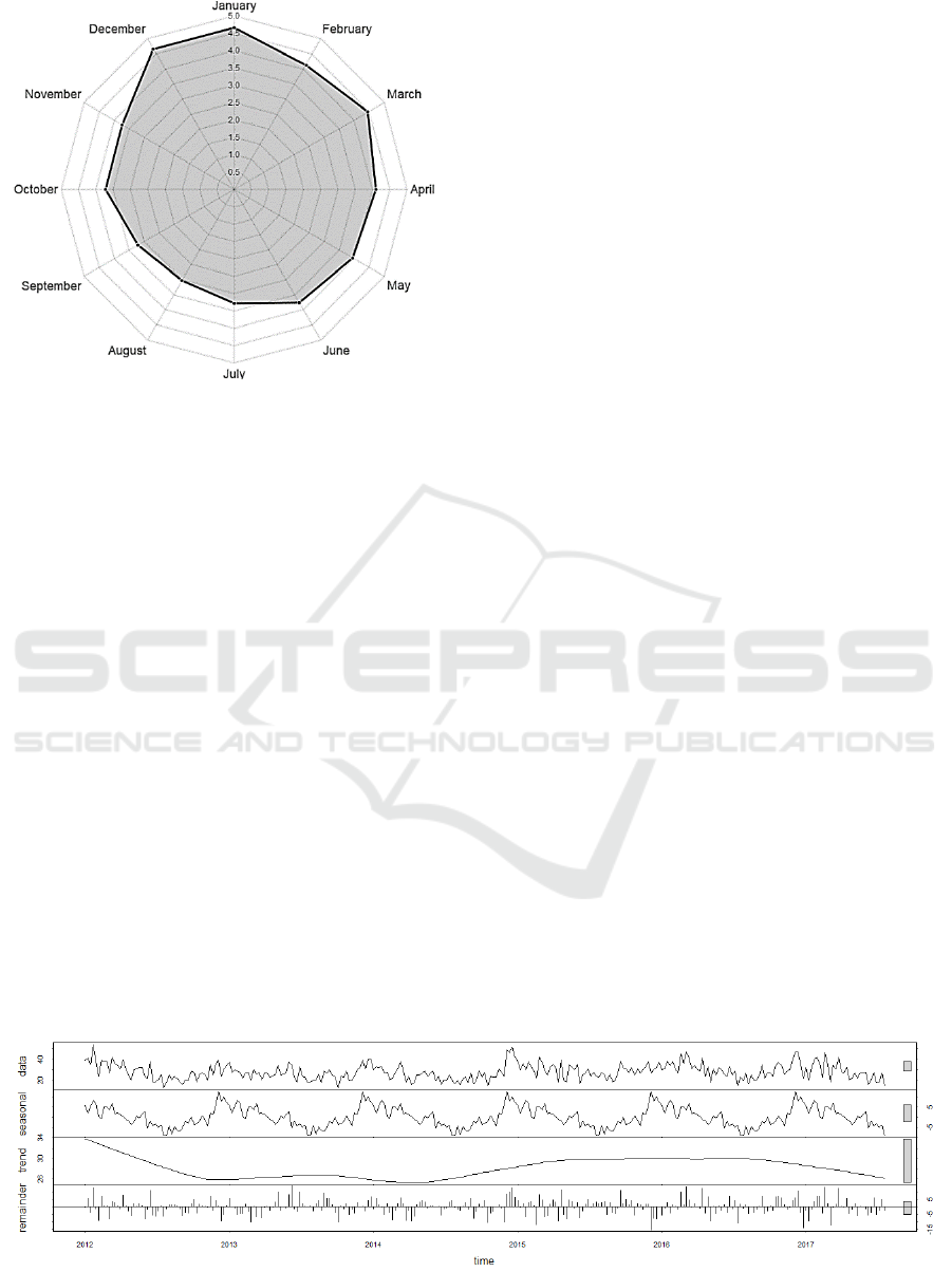
Figure 1: Average number of admissions per day in each
month.
4.1 Grouping
Note that the number of hospitalizations per day is
4.02 (Section 3.1). This is not a sufficient number to
analyse the data within each day. Therefore, each
attribute of the study was grouped by weeks: on the
one hand, admissions related data is grouped by the
total number of admissions in each week. On the
other hand, the mean, maximum, minimum and the
standard deviation of each week are used to group the
environmental attributes.
Once the data was grouped by weeks, two different
studies were done: (i) a univariate regression to
determine whether the admissions may influence
future hospitalizations’ prediction (Section 4.2), and
(ii) a multivariate regression to determine the impact
of environmental factors on admission rates (Section
4.3).
4.2 Univariate Regression
In order to study the effect of admissions in future
hospitalizations rate, firstly time series
decomposition is performed (Section 4.2.1) as
exploratory data analysis. Secondly, the best
univariate ARIMA model is tentatively identified and
finally determined (Section 4.2.2).
4.2.1 Decomposition
The hospitalization rate may vary on time depending
on several factors. In order to determine how these
variations behave, a decomposition process was
conducted. This is a mathematical procedure which
transforms a time series into three components, each
of them depicting one of the underlying categories of
patterns: seasonality, trend and random (Jebb and
Tay, 2017). Seasonality represents patterns that are
repeated in a fixed period of time (e.g. repeating
pattern over years). Trend is the underlying tendency
of the data, and random is the residuals of the original
time series after the extraction of the seasonality and
trend, which is also called noise or reminder.
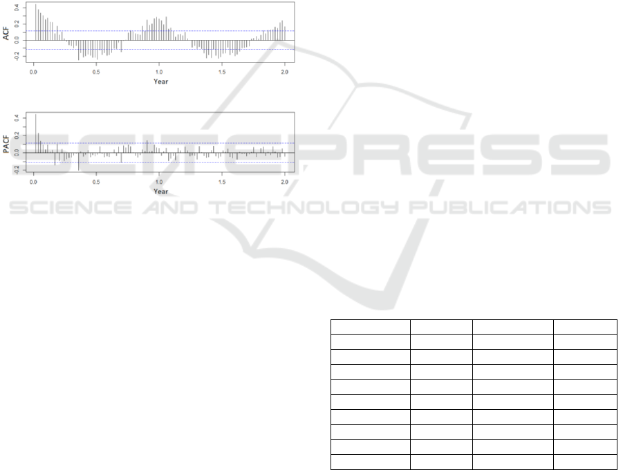
In Figure 2 the decomposition of admissions on
these three components is shown. The first graph
represents the original admissions data series, and
below the seasonality of it is illustrated. Next,
admissions’ trend is presented, and the last graph
reflects the random part of the time series after the
extraction of seasonality and trend components.
Figure 2 shows a clear seasonality of admissions,
since there is a similar pattern every year. In addition,
the tendency represented in the third graph shows
changes in the number of admissions over time.
4.2.2 Univariate ARIMA
Once the decomposition was done, the
hospitalizations dataset was analysed as time series to
determine the impact of admissions on following
week’s hospitalizations. For that, the ARIMA model
was implemented.
ARIMA stands for auto-regressive integrated
moving average and it is a class of statistical models
for analysing and forecasting time series data
Figure 2: Decomposition of admission data series.
HEALTHINF 2019 - 12th International Conference on Health Informatics
54
(Jenkins, 2014) It is specified by three order
parameters: the auto-regressive (AR) parameter p,
which specifies the number of time lags used in the
model; the d represents the degree of differencing
(subtracting its current and previous values d times)
in the integrated component (I); and the order q of the
moving average component (MA) determines the
number of terms to include in the model.
However, to determine the values of the order
parameters p, d, q the autocorrelation function (ACF)
and the partial autocorrelation function (PACF) were
computed (Jain and Mallick, 2017). Figure 3,
represents the ACF and PACF of admissions,
considering the 53 weeks of a year. It shows that there
is a correlation between the number of admissions in
a week with the adjoining precedent weeks and with
the week of the previous years.
Figure 3: Autocorrelation (ACF) and partial autocorrelation
(PACF) plots of admissions.
The smooth decreasing shape of the ACF graph
points at the AR as the best model to be applied in
ARIMA (Jebb and Tay, 2017).
However, to obtain an optimal result to estimate the
likelihood of a model to predict the future values,
different values for p, d, q were tested. For that
selection we took into account the Akaike
information criterion (AIC), from which the one that
presents the minimum AIC value was considered the
optimal (Akaike, 1974). The results showed that
ARIMA (p, d, q) = (0,1,1) got the best results
(minimum AIC).
Once these ARIMA orders were established, it was
essential to determine whether the information
extraction was performed correctly. This process
occurs in two steps: (1) visually examining an ACF
and PACF of the residuals, and (2) conducting a
Ljung-Box test. In the visual analysis of the ACF and
PACF of the residuals a significant correlation was
observed every two months. As expected, in the
widely used formal test of Ljung-Box test (Ljung and
Box, 1978), applied in our study, we saw that there
was still some remaining information extractable (p-
value = 0.028), caused by the remaining correlation
observed in the residuals every two months.
However, it has not been possible to extract further
information.
4.3 Multivariate Regression
The next step was to analyse the regression taking
also into account the environmental information. To
do that, the first step was to calculate the correlations
between all environmental factors and admission
rates. This way we could select the most significant
factors for the experiment. Following, the
multivariate ARIMA was implemented to determine
their impact all together.
4.3.1 Selection of Attributes
As mentioned before, the variables were grouped by
weeks (see Section 4.1).
The correlation was estimated using the non-
parametric test of Kendall, which measures the
strength of dependence between two numeric
variables (Rui and Vera, 2017) and it is one of the
most used test for this type of non-parametric data. In
addition, this analysis was done relating all the
attributes with the number of admissions of the
following week.
Note that, since the mean, maximum and minimum
values of the environmental factors were closely
related, only the one with the highest correlation was
taken into account per attribute. In Table 3 we
summarize the selected ones.
Table 3: Selected attributes for the experiment.
Attribute
Selected
Correlation
p-value
Humidity
Max
0.0469
0.2381
Precipitation
Mean
0.0795
0.0461
Temperature
Mean
-0.3794
1.44E-21
Irradiation
Mean
-0.2629
3.88E-11
NO
Max
0.2107
1.82E-07
NO
2
Mean
0.1876
1.95E-05
NOX
Max
0.2196
4.06E-08
PM10
Min
-0.0485
0.3243
SO
2
Max
0.2692
3.17E-09
Table 3 shows that the most correlated attribute
was the temperature, showing the highest (inversed)
correlation value. This shows that the lower the
temperature, the larger is next week admission rate.
On the other hand, humidity, precipitation, and PM10
parameters do not have significant correlations in this
study, neither relevant p-values.
The Impact of Environmental Factors on Heart Failure Decompensations
55

Besides this analysis, environmental factors
variations, such as temperature variations, might also
affect the health status. Therefore, the impact of the
highest temperature change per week, and the
standard deviation (SD) of each attribute per week
were also studied following the same procedure
(Table 4).
Table 4 shows that the temperature change does not
affect in the next week’s admission rate. However,
some attributes’ instability (standard deviation) over
the week seems to be correlated. Hence, the standard
deviation of the attributes Irradiation, NO, NOX and
SO2 will be checked in the multivariate ARIMA
regression.
Table 4: Correlations of the attributes’ standard deviations
and the temperature change.
Attribute SD
Correlation
p-value
Humidity
0.05
0.25
Precipitation
0.06
0.11
Temperature
0.03
0.39
Irradiation
-0.20
4.13e-07
NO
0.23
1.54e-08
NO
2
0.06
0.18
NOX
0.20
3.73e-07
PM10
0.02
0.75
SO
2
0.23
1.58e-07
Temp. change
0.04
0.26
4.3.2 Multivariate ARIMA
Using the model extracted from the univariate
ARIMA analysis and after the selection of the most
correlated environmental attributes, a multivariate
ARIMA model was carried out.
For that, first we employed all attributes and tested
the AIC value. If the p-value of an attribute was too
high, this value was discarded, and the AIC value was
checked again. If the value improved (AIC
decreased), we kept that value out of our model.
Otherwise we put it back. This process was done
iteratively until AIC did not decrease anymore.
5 RESULTS
In this chapter, the results obtained from univariate
and multivariate ARIMA regressions are presented.
On the one hand, univariate ARIMA shows an AIC
value of 1939.71, with p-values of <2.2e-16 for MA1
(moving average order 1 of admissions) and <6.248e-
8 for SMA1 (seasonal moving average order 1 of
admissions). It is noticeable that the result obtained is
quite precise.
Even so, adding the environmental variables
(multivariate ARIMA), it was found to be possible to
improve the predictive power of the model. At the
beginning, it was tested with all the attributes, slightly
improving the result (AIC of 1631.6). After a filtering
of attributes depending on their p-value, the optimal
model was achieved with an AIC of 1620.59. This last
model is represented in Table 5 with their respective
p-values for each variable.
Table 5: Results of the multivariate ARIMA model study.
Significant codes: 0 ‘***’, 0.001 ‘**’, 0.01 ‘*’.
Variable
Estimate
Std.
Error
p-value
ma1
1
-0.9230
0.0258
< 2.2e-16 ***
sma1
2
-0.7075
0.1192
2.929e-09 ***
Mean
Precip.
-0.2935
0.1189
0.0136 *
Mean
Temp.
-0.6056
0.1865
0.0012 **
Max. SO
2
0.3171
0.1176
0.007**
Std. NOX
-0.0797
0.0342
0.0197 *
1
Moving average order 1 of admissions
2
Seasonal moving average order 1 of admissions
As shown in Table 5, the attribute with most impact
on the number of admissions is the admissions itself.
This is reflected in the variables called “ma1” and
“sma1”, which are the moving average and the
seasonal moving average (season of a year)
respectively. Nevertheless, environmental factors
also have a considerable influence. For example, the
model predicts that when the mean temperature rises
1
o
C the estimated number of hospitalizations will
decrease by 0.6 (when the rest of attributes remain
constant). Moreover, the maximum value for SO
2
within a week also has an effect (p-value = 0.007).
Additionally, the variability of air quality parameter
(NOX) also presents an impact on admissions
predictions. Finally, the results also present that the
more it rains, the less number of hospitalizations
occur the following week.
The mean air temperature, which has high impact
on admission rate prediction (see Table 5), is
represented in a more visual way by comparing the
number of admissions per weeks with the mean
temperature, using a line graph (see Figure 4).
HEALTHINF 2019 - 12th International Conference on Health Informatics
56
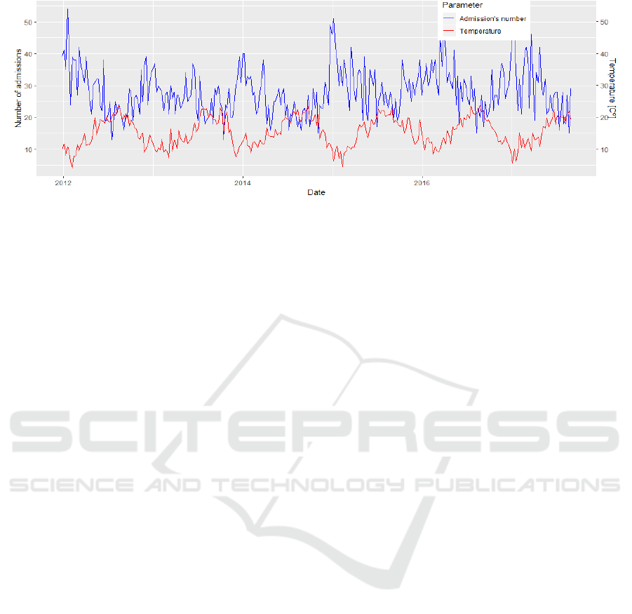
Figure 4: Comparison between the number of admissions (in blue) and the mean temperature (in red) per week over time.
6 CONCLUSIONS AND FUTURE
GUIDELINES
In this paper, the impact of different environmental
factors on Heart Failure (HF) decompensations by
means of hospital admissions is studied. For that, a
regression model for time series was built, and the
external attributes that most affect the number of
hospitalizations were tested. In this context, air
temperature was concluded to be the most significant
environmental factor, although some other attributes,
such as precipitation, along with SO
2
and NOX air
quality parameters, were also demonstrated to be
relevant.
In the future, these environmental factors will be
included on already built predictive models to assess
the risk of decompensation of an ambulatory patient
(Larburu et al., 2018). This model predicts the
decomposition risk within seven days, using the
previous days’ monitoring data of the patients.
Adding the environmental factors described in this
study may improve its predictiveness.
Moreover, despite the objective of the study was to
just detect environmental attributes influence in the
HF patients’ decompensations, a predictive model to
predict the admissions’ number of the following week
could be developed. This could be very useful for the
physicians to anticipate a possible bed over-
occupancy situation in hospitals. A first test of this
model has been conducted with ARIMA predicting
model. It predicts with a mean error of 4 admissions
each week (when the number of hospitalizations per
week is 28). Nevertheless, this testing error is
achieved using the same dataset for training and for
testing. Hence, unless it is not tested in a new dataset,
the results cannot be generalized. Therefore, this test
remains as future work.
ACKNOWLEDGEMENTS
This work has been funded by the Basque
Government by means of Hazitek Program, under
eCardioSurf project and by Gipuzkoako Foru
Aldundia under MANAVICO proyect.
REFERENCES
Akaike, H., 1974. A new look at the statistical model
identification. IEEE Trans. Autom. Control 19, 716–
723.
Angelini, F. et al., 2017. The Impact of Environmental
Factors in Influencing Epigenetics Related to Oxidative
States in the Cardiovascular System. Oxid. Med. Cell.
Longev.
Basque Government, B.G., 2009. Open Data Euskadi,
datos abiertos del Gobierno Vasco - Euskadi.eus. URL
http://opendata.euskadi.eus/inicio/ (accessed 9.18.18).
Benjamin, E.J. et al., 2016. Heart Disease and Stroke
Statistics-2016 Update: A Report From the American
Heart Association. Circulation 133, e38-360.
Brook, R.D. et al., 2004. Air Pollution and Cardiovascular
Disease.
Brook, R.D. et al., 2010. Particulate matter air pollution
and cardiovascular disease: An update to the scientific
statement from the American Heart Association.
Circulation 121, 2331–2378.
Burnett, R.T., Dales, R.E., Brook, J.R., Raizenne, M.E.,
Krewski, D., 1997. Association between Ambient
Carbon Monoxide Levels and Hospitalizations for
Congestive Heart Failure in the Elderly in 10 Canadian
Cities. Epidemiology 8, 162–167.
D’Amato, G., Cecchi, L., D’Amato, M., Liccardi, G., 2010.
Urban air pollution and climate change as
environmental risk factors of respiratory allergy: an
update. J. Investig. Allergol. Clin. Immunol. 20, 95–
102; quiz following 102.
The Impact of Environmental Factors on Heart Failure Decompensations
57

Das, D. et al., 2014. The association between
meteorological events and acute heart failure: New
insights from ASCEND-HF. Int. J. Cardiol. 177, 819–
824.
Gobierno Vasco, E.J., 2017. Calidad del aire en Euskadi
durante el 2017. URL
http://www.geo.euskadi.eus/calidad-aire-en-euskadi-
2017/s69-geodir/es/ (accessed 5.17.18).
Gurría, A., 2012. OECD Environmental Outlook to 2050 -
The Consequences of Inaction. OECD. URL
http://www.oecd.org/env/indicators-modelling-
outlooks/oecd-environmental-outlook-1999155x.htm
(accessed 9.26.18).
Heidenreich, P.A. et al., 2011. Forecasting the Future of
Cardiovascular Disease in the United States.
Circulation.
Jain, G., Mallick, B., 2017. A Study of Time Series Models
ARIMA and ETS (SSRN Scholarly Paper No. ID
2898968). Social Science Research Network,
Rochester, NY.
Jebb, A.T., Tay, L., 2017. Introduction to Time Series
Analysis for Organizational Research: Methods for
Longitudinal Analyses. Organ. Res. Methods 20, 61–
94.
Jenkins, G.M., 2014. Autoregressive–Integrated Moving
Average (ARIMA) Models, in: Wiley StatsRef:
Statistics Reference Online. American Cancer Society.
Larburu, N., Artetxe, A., Escolar, V., Lozano, A., Kerexeta,
J., 2018. Artificial Intelligence to Prevent Mobile Heart
Failure Patients Decompensation in Real Time:
Monitoring based Predictive Model. Indawi.
Laumbach, R.J., Kipen, H.M., 2012. Respiratory health
effects of air pollution: Update on biomass smoke and
traffic pollution. J. Allergy Clin. Immunol. 129, 3–11.
Levin, R.K., Katz, M., Saldiva, P.H.N., Caixeta, A.,
Franken, M., Pereira, C., Coslovsky, S.V., Pesaro, A.E.,
2018. Increased hospitalizations for decompensated
heart failure and acute myocardial infarction during
mild winters: A seven-year experience in the public
health system of the largest city in Latin America. PLOS
ONE 13, e0190733.
Ljung, G.M., Box, G.E.P., 1978. On a measure of lack of fit
in time series models. Biometrika 65, 297–303.
Moritz, S., Bartz-Beielstein, T., 2017. imputeTS: Time
Series Missing Value Imputation in R. R J. 9, 207–218.
Morris, R.D., Naumova, E.N., Munasinghe, R.L., 1995.
Ambient air pollution and hospitalization for
congestive heart failure among elderly people in seven
large US cities. Am. J. Public Health 85, 1361–1365.
Ponikowski, P. et al., 2014. Heart failure: preventing
disease and death worldwide. ESC Heart Fail. 1, 4–25.
Rui, S., Vera, C., 2017. Comparative Approaches to Using
R and Python for Statistical Data Analysis. IGI Global.
Stewart, S., McIntyre, K., Capewell, S., McMurray, J.J.V.,
2002. Heart failure in a cold climate: Seasonal
variation in heart failure-related morbidity and
mortality. J. Am. Coll. Cardiol. 39, 760–766.
Warren, R., Walker, B., Nathan, V.R., 2002. Environmental
factors influencing public health and medicine: policy
implications. J. Natl. Med. Assoc. 94, 185–193.
Woolf, S.H., Aron, L., 2013. Physical and Social
Environmental Factors. National Academies Press
(US).
HEALTHINF 2019 - 12th International Conference on Health Informatics
58
