Reinforcement Learning Approach for Cooperative Control of

Multi-Agent Systems

Valeria Javalera-Rincon

, Vicenc Puig Cayuela

, Bernardo Morcego Seix

and

Fernando Orduña-Cabrera

Advanced Systems Analisys and Ecosystem Services and Management Programs, International Institute for Applied

Systems Analysis, Schlossplatz 1, A-2361, Laxenburg, Austria

Advanced Control Systems Group, Universitat Politècnica de Catalunya (UPC), Rambla Sant Nebridi, 10,

08222 Terrassa, Spain

Keywords: Distributed Control, Intelligent Agents, Reinforcement Learning, Cooperative Agents.

Abstract: Reinforcement Learning (RL) systems are trial-and-error learners. This feature altogether with delayed

reward, makes RL flexible, powerful and widely accepted. However, RL could not be suitable for control of

critical systems where the learning of the control actions by trial and error is not an option. In the RL literature,

the use of simulated experience generated by a model is called planning. In this paper, the

planningByInstruction and planningByExploration techniques are introduced, implemented and compared to

coordinate, a heterogeneous multi-agent architecture for distributed Large Scale Systems (LSS). This

architecture was proposed by (Javalera 2016). The models used in this approach are part of a distributed

architecture of agents. These models are used to simulate the behavior of the system when some coordinated

actions are applied. This experience is learned by the so-called, LINKER agents, during an off-line training.

An exploitation algorithm is used online, to coordinate and optimize the value of overlapping control variables

of the agents in the distributed architecture in a cooperative way. This paper also presents a technique that

offers a solution to the problem of the number of learning steps required to converge toward an optimal (or

can be sub-optimal) policy for distributed control systems. An example is used to illustrate the proposed

approach, showing exciting and promising results regarding the applicability to real systems.

1 INTRODUCTION

RL is a well-known and formally studied family of

learning techniques. Moreover, depending on the

formulation of the problem and the richness of

experience data, the chances of convergence are high.

One of the main characteristics of RL is that the

agents learn by trial and error discovering which

actions yield the maximum reward by trying them.

However, it is also this characteristic what makes RL

unsuitable for controlling critical time-varying

systems where good performance is crucial all the

time, and the cost of this learning curve of the agent

can be too high.

Currently, some algorithms implement planning

techniques such as Dyna-Q and Prioritized Sweeping.

Some examples of applications of Dyna-Q algorithm

are (Tateyama et al. 2007), (Hwang et al. 2015) and

(Hwang et al. 2017). Moreover, for Prioritized

Sweeping see (Zajdel 2018) and (Desai and Patil

2017). In these cases, the planning techniques are

used to simulate experience generated by a model.

Here two planning techniques are introduced aiming

to work cooperatively and coordinated getting a

heterogeneous multi-agent architecture for Large

Scale Systems (LSS).

These planning techniques were specially

developed to fit into the LINKER Architecture (LA)

introduced in (Javalera 2016) as the MA-MPC

architecture. First descriptions and applications of

this architecture were presented in (Javalera et al.

2010), and the use of this architecture and

methodology to the Barcelona Drinking Water

Network is described in (Morcego et al. 2014). In all

these applications the agents implement a control

technique called "Model Predictive Control (MPC),"

therefore the name of the architecture. However, this

work is called LINKER architecture, since the

algorithms and architecture can be applied to other

types of agents as well, not just MPC.

Reinforcement learning (RL) works based on

experience, which, in LA is used aiming to reduce the

Javalera-Rincon, V., Cayuela, V., Seix, B. and Orduña-Cabrera, F.

Reinforcement Learning Approach for Cooperative Control of Multi-Agent Systems.

DOI: 10.5220/0007349000800091

In Proceedings of the 11th International Conference on Agents and Artiﬁcial Intelligence (ICAART 2019), pages 80-91

ISBN: 978-989-758-350-6

requirement of iterative methods, facilitating that the

system behaves almost like a reactive system with

reduced response time. Another relevant feature of

RL exploited by the LINKER Architecture is that it

explicitly considers the whole problem of a goal-

directed agent interacting with an uncertain

environment. Moreover, this is in contrast with many

approaches that consider sub-problems without

addressing how they might fit into a larger picture.

Even more, this is important for the LINKER

Architecture because it is distributed control

architecture of LSS, where some of its control

variables overlap between sub-systems; this issue is

aboard in the next section.

This paper aims to explain how using the

proposed learning techniques and the LINKER

Architecture, and is possible to integrate agents of a

distributed system with LINKER agents trained with

the proposed planning techniques. Each LINKER

agent calculates the value of shared variables between

overlapping systems looking for the global optimum

of the relation and coordinating its process with the

other agents of the system obtaining an overall good

performance. This work also proposes a solution that

makes possible to achieve the benefits of RL

techniques in critical systems that cannot afford to

pay the learning curve of a learner agent. Even more,

this is made using a meaningful reinforcement given

by the distributed agents that try the actions in its

internal model in offline training. Once all the

functions learned are evaluated and approved, the

LINKER agents use an online optimization algorithm

that can also have adaptation properties.

Another contribution of this paper is to compare

two learning techniques. In the first one, the actions

used in training are dictated by a teacher that, in this

case, is the centralized MPC (Model Predictive

Control) controller. In second one a learning

technique where actions are randomly selected. The

LINKER agent explores actions trying and evaluating

it, through the interaction with the agents that directly

control the model. An illustrative example is

developed using both techniques.

The structure of the paper is as follows: Section 2

introduces the problem statement. Section 3 presents

the model driven control and the model driven

integrated learning. Section 4 presents the planning

by instruction while Section 5 presents the planning

by exploration. Section 6 uses an application case

study to illustrate the performance of the proposed

architecture and approaches. Finally, Section 7

summarizes the main conclusions and describes the

future line of research.

2 PROBLEM STATEMENT

In order to describe the learning techniques

mentioned above, it is necessary to explain the

underlying problem, which is the distributed control

problem that the LINKER architecture addresses.

This architecture is applied to a LSS.

In order to control an LSS in a distributed way,

some assumptions have to be made on its dynamics,

i.e. on the way the system behaves. Let us assume first

that the system can be decomposed into n sub-

systems, where each sub-system consists of a subset

of the system equations and the interconnections with

other sub-systems. The problem of determining the

partitions of the system is not addressed in this work.

The set of partitions should be complete. This means

that all system states and control variables should be

included at least in one of the partitions.

Definition 1. System partitions. P is the set of

system partitions and is defined by

 







 



  





(1)

Where each system partition (subsystem) 



,  



  



is described by a model. In this example, a

deterministic linear time-invariant (LTI) model is

used to represent a drinking water distribution

network; this type of model can also be used for other

type of LSS where there is a network of connected

nodes and an element that flows in the network that

should be distributed to fulfill certain demands. This

model is expressed in discrete-time as follows







  



 













 









 























 













 













 













(2)

The model describes the topology and dynamics

of the network. Variables x, y, u, d are the state,

output, input and disturbance vectors (for this case,

the demands) of appropriate dimensions,

respectively; A, B, C and D are the state, output, input

and direct matrices, respectively. Sub-indexes u and

d refer to the type of inputs the matrices model, either

control inputs or exogenous inputs (disturbances).

Control variables are classified as internal or shared

variables.

Reinforcement Learning Approach for Cooperative Control of Multi-Agent Systems

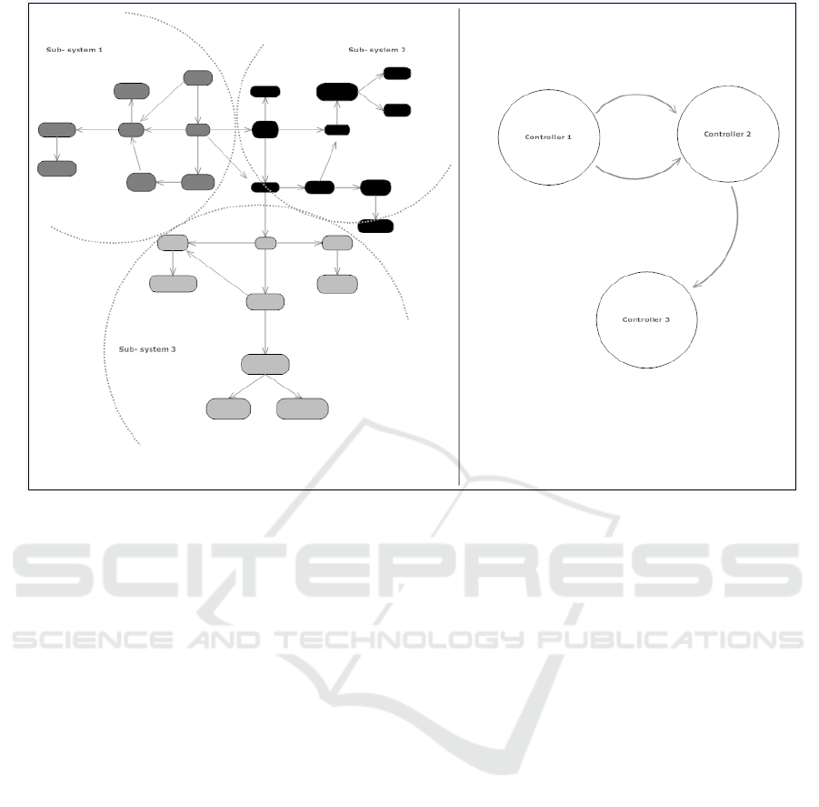
Figure 1: The problem of distributed control.

Definition 2. Internal Variables. Internal variables

are control variables that appear in the model of only

one subsystem in the problem. The set of internal

variables of a partition i is defined by equation 3:





 



 



  



}

(3)

Definition 3. Shared Variables. Shared variables are

control variables that appear in the model of at least

two subsystems in the problem. Their values should

be consistent in the subsystems they appear. They are

also called negotiated variables because their values

are obtained through a negotiation process. 



is the

set of negotiated variables between partitions i and j,

defined by equation 4





 



 



  





(4)

Each subsystem i is controlled by a controller (agent)

using:

 the model of the dynamics of subsystem i given

by eq. (2);

 the measured state x

(k) of subsystem i;

 the exogenous inputs d

(k) of subsystem i over a

specific horizon of time;

As a result, each agent calculates directly the

internal control actions, u

(k), of subsystem i. Figure.

1 on the left shows a sample system divided into three

partitions. Subsystem 1 has two shared variables with

sub-system 2 and subsystem 2 has one shared variable

with sub- system 3. The relations that represent those

variables are shown on the right as lines. The problem

consists in optimizing the manipulated variables of

the global system using a distributed approach, i.e.

with three local control agents that should preserve

consistency in the shared variables. In order to solve

the problem described above, a new framework has

been developed. This framework comprises a

methodology, the so called the LINKER

methodology and the architecture. The methodology

helps to implement the architecture

3 A MODEL DRIVEN CONTROL

AND A MODEL DRIVEN

INTEGRATED LEARNING

The LINKER architecture integrates a model driven

control and a model driven learning process. In order

to perform the negotiation of the shared variables, the

Linker agent learns to think globally, by means of an

offline training where negotiator and agents interact

and accumulate meaningful experience. This offline

training is made using a model of each sub-system

environment computing value functions (Q-tables)

whose optimality and efficiency are proved in the

experimentation phase, in order to be used later in the

ICAART 2019 - 11th International Conference on Agents and Artiﬁcial Intelligence

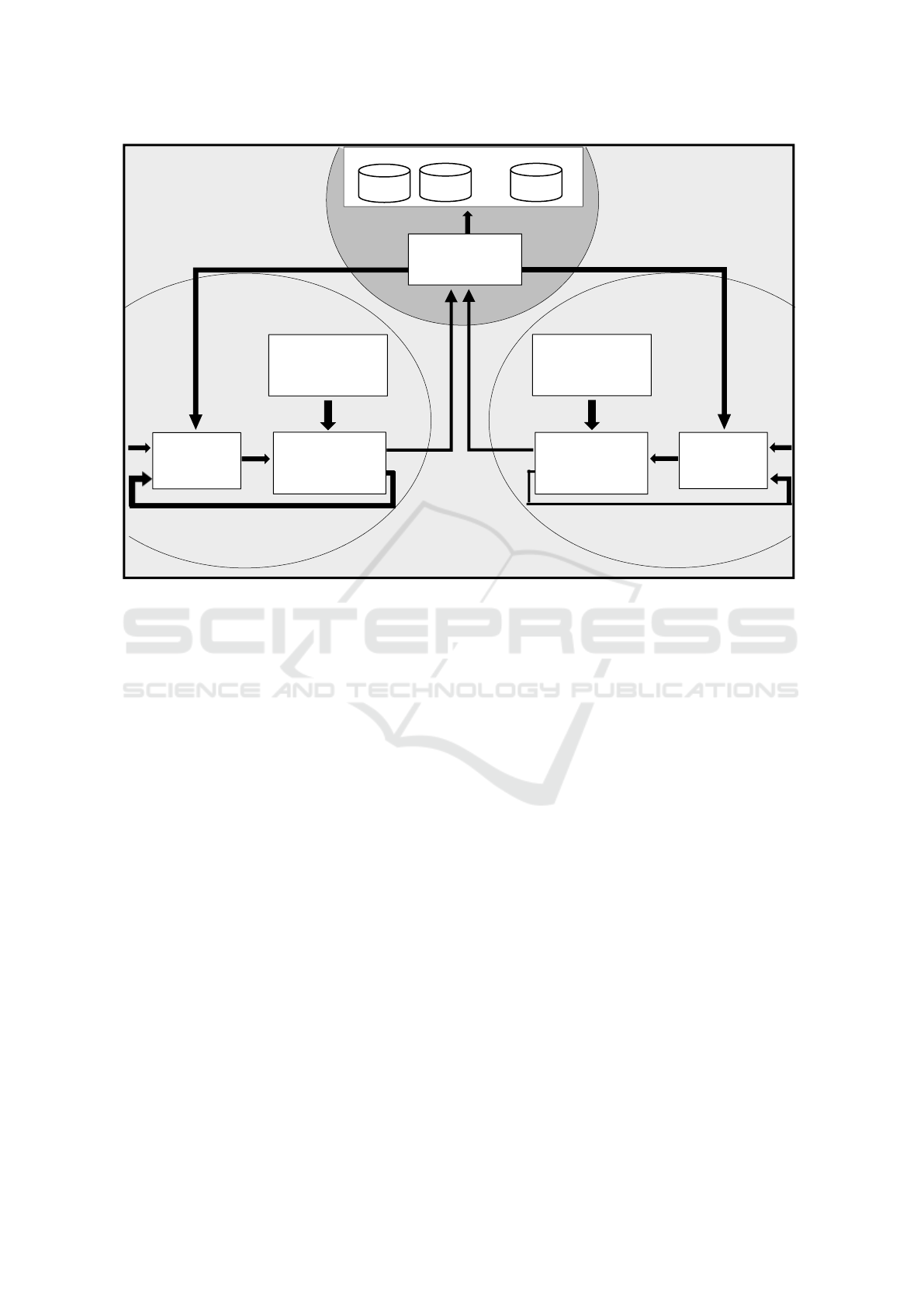
Figure 2: Integration of the models of agents in the planning process.

negotiation process. This allows eliminating iterative

communication between agents in the negotiation

process, increasing efficiency, decreasing time of

response and making it safe to implement.

Figure 2 shows the integration of the models in the

agents in the planning process. The Linker agent

assigns the values of V to the related agents. Each

related agent has its own reference, disturbance model

and plant model according to Eq. 2. The local

controller takes V as constraints, computes vector c and

applies the control action to the plant model producing

y and e. e is an error vector that indicates to the Linker

how good the actions (V) were. In order to evaluate that,

it is necessary to calculate the state of both agents. This

is made based in the cost function of the agents, as for

example,

s1= Hpi=0J(i)= Hpi=0Jx (i)+ Hpi=0 Ju(i)

(5)

s2= Hpi=0J(i)= Hpi=0Jx (i)+ Hpi=0 Ju(i)

(6)

where





  

















 and





   



















(7)

The reward (r), is calculated using the states of

both MPC agents with the equation:

    



 



(8)

where  represents the reward r and  is a constant

that satisfies:





 



 

(9)

Given that s

and s

represents a sum of quadratic

errors (5), (6), the reward will be always positive.

With a smaller sum of errors the reward will be larger

and vice versa. s

and s

have to be discretized in order

to be use in









 





  







 





(10)

that is the function that updates each Q-table where

the parameters  rates past experience.

The purpose of this three-dimensional matrix is to

map the state agent 1 (



) and the state of agent 2 (



)

to a single action. The coordination feature of the

Linker agent lies on the fact that, in exploitation, the

Linker agent will map to an optimal (or sub-optimal)

action every 



and



eliminating with this conflicts

between agents assigning the value of shared

variables.

The Linker uses this simulated experience and

updates the Q-values in the Q-tables, one for each

shared variable of the vector V in order to improve its

policy. All this process is implemented through the

PlannigByInstruction and PlanningByExploration

…

Local

controller

Disturbance

Model 1

agent1

agent2

LINKER

Local

controller

Plant Model 2

Disturbance

Model 2

Plant Model 1

Planning

Reinforcement Learning Approach for Cooperative Control of Multi-Agent Systems

behaviors of the Linker that will be explained in

further detail in next section.

The integration of RL with the LTI model in this

approach offers high cohesion to the system. The

support that the LTI model (2) offers is deterministic,

descriptive and highly trusted. So, the integration of

these techniques coupled by the implementation of

the methodology makes the planning process efficient

and reliable.

The policy obtained is evaluated in the

experimentation phase. The fact that the policy is

obtained offline is a very important characteristic of

this approach due to the critical nature of LSS. The

use of a standard trial-and-error technique of RL

would make the implementation of this approach

unfeasible. If the learning process is driven from real

experience in the plant, the system will be unfeasible

most of the time at the beginning of the process and

the actuators can be damaged. That is why, in this

framework, in order to arrive to the implementation

phase, the optimality of the obtained policy has to be

tested beforehand.

4 PLANNING BY INSTRUCTION

In contrast to some IA learning methods, like

supervised learning, in this work, the term instruction

refers to the way in which the action is selected in the

learning process, and not to the type of the feedback

used. So, PlannigByInstruction behavior (PBIB) is a

learning behavior that implements a specific

combination of choosing actions and providing

feedback.

4.1 Description of the Approach

The purpose of this learning behavior is to obtain an

optimal policy (Q), constructing a knowledge base

based on the evaluation of actions given by a teacher.

This teacher has to be a trustable controller, like a

centralized MPC or the actions taken by a human

expert. These actions are simulated in the model

system and the result (states s

and s

, (5), (6)) is

evaluated obtaining a reward (r) (8) that is used to

obtain the new Q-value (10). n

iterations are made

for the complete control horizon with random initial

conditions. This behavior is performed offline in the

training phase of the LINKER methodology.

Assuming that there is a single negotiation variable,

the PlanningByInstruction behavior algorithm

describes the training algorithm that the NA executes

in order to update its Q-table by this learning behavior

In this algorithm, s

and s

represents the states

(5), (6) of agent1 and agent2 (the two agents that

share that particular negotiation variable). V

and V

are the internal representations of the shared variable

in Agent1 and Agent2 (sub-indices a1 and a2

respectively) for k instant. teacherAction is the action

dictated by the teacher.

Define , n, s

← random, s

← random,

controlHorizon, teacherAction (1-control horizon), k=1

loop while iterations ≤ n

loop while k ≤ controlHorizon

(k) ← teacherAction (k)

← send V

(k) to agent1, agent1 set the

action V

(k) and calculates its internal variables,

apply all the controls (actions) obtained (and

given) for step k to its LTI model of its partition

and calculates s

using

(5)

← send V

(k) to agent2, agent2 set the

action V

(k) and calculates its internal variables,

apply all the controls (actions) obtained (and

given) for step k to its LTI model of its partition

and calculates s

using

(6)

r ← - s

- s

Q (s

’, teacherAction (k)’, s

’ )← r +α Q(s

teacherAction (k), s

)

’← s

k=k+1

end loop

iterations=iterations+1

end loop

5 PLANNING BY EXPLORATION

Learning by exploration is the main type of learning

technique used in RL. It is based on trying random

actions from a deterministic and finite set, in order to

obtain a feedback that represents how good the taken

action was. Learning by exploration in LSS can be a

difficult task because of the size and complexity of

these systems. The PlanningByExploration behavior

(PBEB) implements learning by exploration

combined with selective feedback. The use of

selective feedback reduces drastically the time of

training needed in order to obtain an optimal policy

(Q) and the difficulty to find a good parameterization

of the learning process in the experimentation phase.

The purpose of this learning behavior is to obtain an

optimal policy (Q), constructing a knowledge base

based on the exploration of a deterministic and finite

ICAART 2019 - 11th International Conference on Agents and Artiﬁcial Intelligence

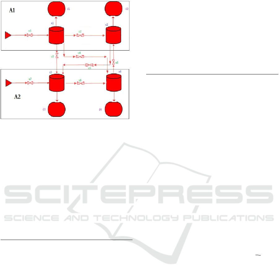
Figure 3: Water network considered as case study.

set of actions. These actions are simulated in the model

system and the result (states s

and s

) is evaluated

and only in case a feasible solution for both agents

(agent1 and Agent2) is found, the feedback is selected

for leaning. For those cases, a reward (r) is obtained

and used to calculate the new Q-value (10). n

iterations are made for the complete control horizon

with random initial conditions. This behavior is

performed offline in the training phase of the LINKER

methodology. Assuming that there is a single

negotiation variable, the PlanningByExploration

behavior algorithm describes the training algorithm

that the LINKER executes in order to update its Q-

table by this learning behavior:

Define , n, s

← random, s

← random,

controlHorizon, k=1

loop while iterations ≤ n

loop while k ≤ controlHorizon

a ← random (a)  A Q (s

′,a, s

′)

(k) ← a

← send V

(k) to agent1, agent1set the action

(k) and calculates its internal variables, apply

all the controls (actions) obtained (and given) for

step k to its LTI model of its partition and

calculates s

using

(5)

← send V

(k) to agent2, agent2set the action

(k) and calculates its internal variables, apply

all the controls (actions) obtained (and given) for

step k to its LTI model of its partition and

calculates s

using

(6)

if agent1 and agent2 have a feasible solution

r ← - s

- s

Q (s

’, a’, s

’ )← r +α Q(s

, a, s

)

’← s

else

’← random

end if

k=k+1

end loop

iterations=iterations+1

end loop

6 ILLUSTRATIVE APPLICATION

This section shows an example of the optimization of

a water distribution network using the proposed

architecture. The partitioning of the network obeys a

geographical criterion, so it has been divided in two

partitions, north and south (see Figure 3). The tanks

and x

will belong to the north sector where a local

control is required. The tanks x

and x

will belong to

the south sector, with its corresponding local

controller.

There are two supply sources and four demand

points, one for each tank. Typically the demands have

a sinusoidal behavior throughout the day that try to

emulate the actual demand behavior. The system shall

operate in a distributed way but looking for global

optimum in the controlled tank levels, satisfying the

demand points of both subsystems, and avoiding

collisions or conflicts among them.

It is expected that the performance of the tank

levels follow a reference variable in time, but without

performing drastic actions in the actuators. The target

control is defined as follows: For each tank (x

, x

) there is a given reference that describes the

desirable behavior of the levels of these tanks. These

levels will be achieved through the manipulation of

the control variables (u

, u

,…,u

) with minor

variations over time.

6.1 Using PBIB

6.1.1 Training

Figure 4 shows a representation of the Q-values

calculated in different phases of the training of the

variable u

. The Q-table contrast the error of M

and

(or the discretize state of each agent) with the

action taken.

In order to use only positive errors, in Fig. 4,

errors range from 0 to 200. Negative errors range

from 0 to 99, 100 corresponds 0 and from 101 to 200

Reinforcement Learning Approach for Cooperative Control of Multi-Agent Systems

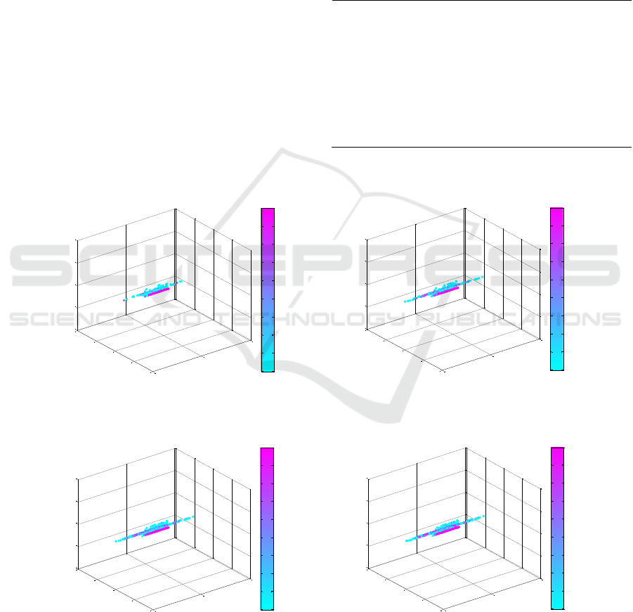
are range the positive errors. Actions are ranging from

0 to 100. As it can be appreciated in the figure, the

states visited in this training tend to be denser near the

optimum state (100). This is because all the actions

were dictated by the teacher, the centralized system.

Making a comparison between sub-figures (a), (b), (c)

and (d) it can be seen that the Q-values cloud is

spreading on the axis of the actions and becomes

denser as the training progresses. It is important to

notice that the only random factor in this training

(using PBIB) are the initial states of A

and A

. The

fact that in this training instructed learning is used

makes it fast and efficient. The Q-values stored in these

Q-tables represents meaningful and evaluated experi-

ence (because of the accumulation of the rewards).

It can be noticed that between section c and d of

the Fig. 4 there is not much difference. This is one of

the factors that can show that no more iterations are

needed. Additionally, the results of the exploitation

phase are necessary in order to determinate that the

training phase is finished. Similar results are obtained

for the rest of the Q-tables. A training based on PBIB

can be also used as a good start (or seed) before a non-

instructed learning technique.

6.1.2 Simulation

As it was mentioned before, in order to know if the

training phase is finished it is necessary to evaluate

the Q-tables making test and exploiting. In order to

do that, the greedy behavior has to be implemented.

The algorithm of greedy behavior is shown below.

Q (s

,a, s

)  s  S, a  A

observe initial state, s

loop

a ←max a ′ A Q (s

′,a, s

′)

← send V

(k) to agent 1

← send V

(k) to agent 2

←s

′

← s

′

end loop

This algorithm observes the state of the agents s

and s

(in a discretized way) and maps it to the action

Q-table Negotiation variable u

training of 50

iterations

(a)

Q-table Negotiation variable u

training of 100

iterations

(b)

Q-table Negotiation variable u

training of 200

iterations

(c)

Q-table Negotiation variable u

training of 300

iterations

(d)

Figure 4: Different phases of the training using PBIB of the variable u5.

100

150

200

100

150

200

Action

QTable Negotiator 1 - Variable u5

Error Agent 1

Error Agent 2

0.9

1.1

1.2

1.3

1.4

1.5

1.6

1.7

x 10

100

150

200

100

150

200

Action

QTable Negotiator 1 - Variable u5

Error Agent 1

Error Agent 2

0.9

1.1

1.2

1.3

1.4

1.5

1.6

1.7

x 10

100

150

200

100

150

200

Action

QTable Negotiator 1 - Variable u5

Error Agent 1

Error Agent 2

0.9

1.1

1.2

1.3

1.4

1.5

1.6

1.7

x 10

100

150

200

100

150

200

Action

QTable Negotiator 1 - Variable u5

Error Agent 1

Error Agent 2

0.9

1.1

1.2

1.3

1.4

1.5

1.6

1.7

x 10

ICAART 2019 - 11th International Conference on Agents and Artiﬁcial Intelligence

that maximizes the accumulated Q-value. Figure 6

shows the resulting actions of the shared variables

applied in the simulations shown above. It can be

notice that the ones calculated by the Linker (blue)

vary les over time than the ones calculated with a

centralized MPC (green). This is archived without

sacrificing performance.

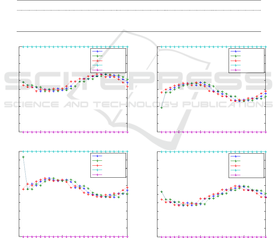
6.1.3 Performance Analysis and Validation

Table 1 shows the average absolute error of the output

of 30 simulations. The first column was calculated

with a training of 50 iterations, next ones with 100

iterations, 200 and 300 iterations. The sum of the

error A

and error A

provides the total error. It can

be seen how the error in the LINKER system (the first

three) decreases as the iterations of the training

progresses. Also it can be noticed that between 200

and 300 iterations there is not much difference in the

error. The analysis of this table and the differences

between the resulting Q-tables is useful to establish

when the training is completed. The results shown in

Figure 5 show, that the LINKER system using

Instructed learning by implementing the

PlanningByInstruction behavior (PBIB) has a better

performance than the centralized MPC solution from

iteration 200.

Table 1: Accumulative ∆u between trainings.





50 it

100 it

200 it

300 it

tralized MPC

4,666e-05

6,333e-05

5,000e-05

6,333e-05

LINKER

0,0140833

0,0153533

0,0116933

0,0155466

Figure 5: Results of the Linker agents (blue) compared with the centralized MPC (green) solution. The red line is the reference,

purple x min, cyan x max.

0 5 10 15 20 25

Time (hr)

Volume (m3)

Agent 1 - Output x1

MA-MPC

Cetralize MPC

Reference

x Max

x Min

0 5 10 15 20 25

Time (hr)

Volume (m3)

Agent 1 - Output x2

MA-MPC

Cetralize MPC

Reference

x Max

x Min

0 5 10 15 20 25

Agent 2 - Output x3

Time (hr)

Volume (m3)

MA-MPC

Cetralize MPC

Reference

x Max

x Min

0 5 10 15 20 25

Agent 2 - Output x4

Time (hr)

Volume (m3)

MA-MPC

Cetralize MPC

Reference

x Max

x Min

Reinforcement Learning Approach for Cooperative Control of Multi-Agent Systems

Table 2: Average of absolute error between increasing

iterations during training with PBIB.





100

200

300

62,36

24,04

18,07

17,14

60,11

24,23

17,20

17,37

LINKER

(PBIB)

122,47

48,27

35,27

34,49

Centralized

MPC

45,91

44,08

45,04

44,71

Table 2 shows the accumulative ∆u objective

applied by the LINKER and the centralized MPC

solution in 30 simulations. The first column was

calculated with a training of 50 iterations, next ones

with 100, 200 and 300 iterations.

The results of this example shows that a system with

multiples dependences between its components can

be governed efficiently using distributed agents and,

even more, it can increase its performance using the

LINKER architecture implementing instructed

learning by the PBIB behavior.

It can also be observed that the actions calculated

by the LINKER (the shared variables) vary less over

time without sacrificing performance. But the

accumulative control effort is minor compared with

the centralized MPC.

Other experiments have been carried varying the

weights of the parameters 



and 



of Eq. (7).

Making the same changes in the teacher (the

centralized MPC) and performing a new training, the

Linker adapts to the new parameterization providing

similar results than ones obtained with the ones used.

6.2 Using PBEB

6.2.1 Training

The training implements the PlanningByExploration

behavior. Many experiments were made in this phase.

First experiments were made using just explorative

learning. Then, the PlanningByExploration behavior

(PBEB) was implemented varying the number of the

iterations in the training. Then, PBEB with selective

penalization of reward was implemented. All

training was made for the complete control horizon

(24 hrs.) for each shared variable. Random initial

conditions were set for each complete horizon.

During training, the Q-table for each shared variable

was filled with the Q-values calculated for all states

visited.

The learning behavior PlanningByExploration,

selects the actions that leads to a feasible solution of

the related MPC agents. In this experiment, PBEB

with selective penalization of reward was

implemented applying a penalization in the opposite

case, this means that if there is no feasible solution for

the local agents, a negative reward was assigned (-

1000). This negative reward ensures that the Q-value

of state-action-state that leads to critical states stays

low and accelerates drastically the training process

allowing the LINKER system to improve the

centralized MPC solution from the iteration 20 (see

Table 3).

Table 3: Comparison of the average absolute error between

local agents, LINKER system and centralized MPC

solution with trainings of 20, 50 and 100 iterations.





20 it

50 it

100 it

17,2429

15,8219

16,3230

18,3069

17,5714

16,3808

LINKER

35,5499

33,3932

32,7038

Centralized

MPC

45,3116

43,7657

42,8805

The experimentation made on this example shows

that using just using exploration, the system cannot

recover from states related to unfeasible solutions. In

addition, these states have high frequency of visits

because it is more likely that the random action

selected were not the good one. This affects

negatively the learning process because the

accumulation of many small rewards becomes in

larges Q-values.

In order to solve that issue, selective feedback

was applied. This reduces drastically the iterations

needed using just exploration and the Q-values

result more reliable. Moreover, the use of a negative

reward in the selected actions that lead to unfeasible

states also provide a huge improvement. After

assigning the negative reward, s’1

and

s’

are set to

random in order to continue the learning process

effectively.

With these conditions a training of 100 iterations

was carried out. Figure 6 (a) shows a color

representation of the Q-values calculated in the

learning process. The Q-table allows to present the

error of A

and A

(or the discretize state of each

agent) with the action taken. In order to use only

positive errors, the errors are scaled from 0 to 200.

Negative errors are scaled from 0 to 99, 100 is 0

while values from 101 to 200 correspond to positive

errors. Actions are ranging from 0 to 100. The

figure compares the Q-tables obtained using PBEB

(a) and (PBIB) (b). From Figure 6 (a), it can be

noticed that the cloud of data spreads all over the

ICAART 2019 - 11th International Conference on Agents and Artiﬁcial Intelligence

action axis, meaning that all actions were explored.

Fig. 6 (b) shows the Q-table of shared variable u

with a training of 300 iterations using PBIB. In this

Q-table, the cloud of Q-values is more compact

because its training only tried the actions dictated by

the teacher (in this case, centralized MPC).

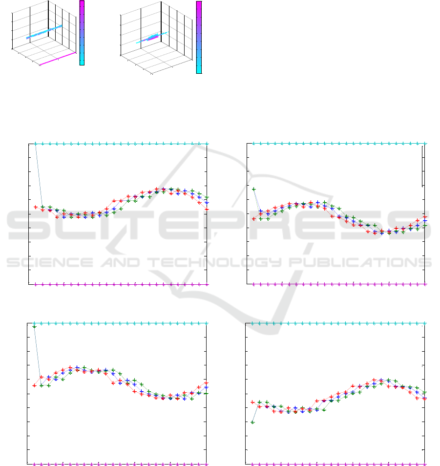
Figure 6: Comparison of the resulting Q-Tables of the

variable u5 using PBEB (a) and PBIB(b).

6.2.2 Simulation

In other to know if the training phase is finished it is

necessary to evaluate the elements of the Q-table by

means of testing and exploiting. The simulation

process implements the greedy behavior (described

above).

The simulation results presented in Figure 7 allow

to compare the LINKER using PBEB (blue line) and

the centralized solution (green line) with the same

random initial conditions and references (red line),

obtained after a training of 100 iterations using PBEB

with selective penalization of reward explained

above. Notice that the reference is variable in time.

The parameters of MPC agents and the centralized

MPC system are the same.

From Figure 7, it can be noticed that both approach

force the system to track the reference.

Figure 7: Results of the MPC agents (blue) compared with the centralized MPC (green) solution. The red line is the reference,

purple x min, cyan x max.

(a)

(b)

100

150

200

100

150

200

Action

QTable Negotiator 1 - Variable u5

Error Agent 1

Error Agent 2

500

1000

1500

2000

2500

3000

3500

4000

100

150

200

100

150

200

Action

QTable Negotiator 1 - Variable u5

Error Agent 1

Error Agent 2

0.9

1.1

1.2

1.3

1.4

1.5

1.6

1.7

x 10

0 5 10 15 20 25

Time (hr)

Volume (m3)

Agent 1 - Output x1

MA-MPC

Cetralize MPC

Reference

x Max

x Min

0 5 10 15 20 25

Time (hr)

Volume (m3)

Agent 1 - Output x2

MA-MPC

Cetralize MPC

Reference

x Max

x Min

0 5 10 15 20 25

Agent 2 - Output x3

Time (hr)

Volume (m3)

MA-MPC

Cetralize MPC

Reference

x Max

x Min

0 5 10 15 20 25

Agent 2 - Output x4

Time (hr)

Volume (m3)

MA-MPC

Cetralize MPC

Reference

x Max

x Min

Reinforcement Learning Approach for Cooperative Control of Multi-Agent Systems

6.2.3 Performance Analysis and Validation

Many simulations were made to assess the

performance of the extended proposed approach.

Table III shows the comparison of the average

absolute error (with respect to the reference) of 30

simulations in the training process of the best Q-

tables found, the ones obtained using PBEB with

selective penalization of reward. Columns show the

results of a training of 20, 50 and 100 iterations with

random reference and initial conditions. From this

table, it can be noticed that the LINKER solution

improves the centralized solution since the first 20

iterations of the training and keeps improving slightly

as iterations increase.

It was observed that the actions calculated by the

Linker (the shared variables) vary less over time

without sacrificing performance. But, the

accumulative control effort is grater compared

with the centralized MPC. Other experiments were

made increasing or decreasing the negative reward

but for this problem the best negative reward was -

1000.

7 CONCLUSION

This article describes three behaviors that

implemented in the LINKER architecture, they

manage to separate the learning process of the

optimization process, eliminating with this the cost

of the number of learning steps necessary to

converge towards an optimal (or can be sub -

optimal) policy.

Explorative training is usually exhaustive. In this

work this complexity is reduced applying selective

feedback (using PBEB) but the combination of the

use of negative reward for the selected feedbacks not

just improves the results compared to the centralized

MPC but also the PlanningByInstruction Behavior

(PBIB) and decrease drastically the iterations

needed in the training phase. Table 4 shows the

average absolute error with respect to the reference

of 30 simulations of the PBEB with selective

penalization of reward and the PBIB. Random initial

conditions and random references were use. The

random cases calculated for PBEB with selective

penalization of reward were different than the ones

calculated for PBIB. The training of the PBEB with

selective penalization of reward, involves 100

iterations while in the case of the PBIB uses 300

iterations.

Table 4: Errors between PBEB with selective penalization

of reward and PBIB.

PBEB selective

reward

PBIB

16,3230

24,04

16,3808

24,23

LINKER

32,7038

48,27

Centralized MPC

42,8805

44,08

Table 5 shows the average 



obtained using the

LINKER and the centralized MPC solution in the

same experimentation conditions that those used to

obtain the results presented in Table 4.

Table 5: Comparison of the J_∆u between the PBEB with

selective penalization of reward and PBIB.

PBEB

PBIB

Centralized MPC

0,0001

6,333e-05

LINKER

0,0107

0,0153533

Thus, the experimentation results obtained in this

example show that PBEB with selective penalization

of reward is a more efficient learning technique than

PBIB due to the reduction of the error and the

iterations needed in training.

The training of the PBEB with selective

penalization of reward and the LINKER framework

was successfully applied into a more realistic case of

study, the Barcelona drinking water network (DWN)

case study (Morcego et al. 2014) and (Javalera et al.

2019). This DWN in managed by Aguas de

Barcelona, S.A. (AGBAR).

ACKNOWLEDGEMENTS

This work was financed by the National Council of

Science and Technology (CONACyT) and PRODEP

of Mexico.

REFERENCES

Desai, R. M. and Patil, B. P., 2017. Prioritized Sweeping

Reinforcement Learning Based Routing for MANETs.

Indonesian Journal of Electrical Engineering and

Computer Science, 5(2), pp.383–390.

Hwang, K., Jiang, W. and Chen, Y., 2017. Pheromone-

Based Planning Strategies in Dyna-Q Learning. IEEE

Transactions on Industrial Informatics, 13(2), pp.424–

435.

Hwang, K.-S., Jiang, W.-C. and Chen, Y.-J., 2015. Model

learning and knowledge sharing for a multiagent system

ICAART 2019 - 11th International Conference on Agents and Artiﬁcial Intelligence

with Dyna-Q learning. IEEE transactions on

cybernetics, 45(5), pp.964–976.

Javalera, V., 2016. Distributed large scale systems: a multi-

agent RL-MPC architecture. Universidad Politécnica

de Cataluña. Available at: http://digital.csic.es/

handle/10261/155199.

Javalera, V., Morcego, B. and Puig, V., 2010. Negotiation

and Learning in distributed MPC of Large Scale

Systems. In Proceedings of the 2010 American Control

Conference. pp. 3168–3173.

Javalera, V., et al. Cooperative Linker for the distributed

control of the Barcelona Drinking Water Network

Proceedings of the International Conference of Agents

and Artificial Intelligence. 2019.

Morcego, B. et al., 2014. Distributed MPC Using

Reinforcement Learning Based Negotiation:

Application to Large Scale Systems. In J. M. Maestre

& R. R. Negenborn, eds. Distributed Model Predictive

Control Made Easy. Dordrecht: Springer Netherlands,

pp. 517–533.

Tateyama, T., Kawata, S. and Shimomura, T., 2007.

Parallel Reinforcement Learning Systems Using

Exploration Agents and Dyna-Q Algorithm. In SICE

Annual Conference 2007. pp. 2774–2778.

Zajdel, R., 2018. Epoch-incremental Dyna-learning and

prioritized sweeping algorithms. Neurocomputing, 319,

pp.13–20

Reinforcement Learning Approach for Cooperative Control of Multi-Agent Systems