Systematic Characterization of a Sequence Group
Paul Irolla
Laboratoire de Cryptologie et Virologie Op
´
erationnelles (CVO Lab),
´
Ecole Sup
´
erieure d’Informatique, d’
´
Electronique et Automatique (ESIEA),
Keywords:
Sequence, Antichain, Android Malware Detection, Clustering, Classification.
Abstract:
Finding similarities in a group of sequences often involves studying their common subsequences or their
common substrings. In our case, Android malware detection/classification, we study the event sequences
coming from the dynamic analysis of applications. For several reasons, these sequences are mostly comprised
of benign events. This specific set up makes classic sequence similarity criteria useless without any machine
learning. The sequence membership to a group is characterized by subsequences of any length. Heuristic
algorithms for extracting short subsequences already exist, but no attempt to solve the problem systematically
has been proposed. We propose a new algorithm for building the Embedding Antichain from the set of common
subsequences (noted A
Γ
). We show that this mathematical representation is very compact and embed all
common subsequences of a sequence set. It is a tool for characterizing a group of sequences. The construction
of this representation reveals several complex subproblems. A few of them are solved in this article, along
with practical implementations. Moreover, we solved different reduced problems and provided suboptimal
solutions for the others. This article opens a new path that has cross-domain applications. Specifically, in the
malware detection/classification domain the Systematic Characterization of Sequence Groups is a tool that can
be used for automatic generation of malware family signatures and detection heuristics. We experimented A
Γ
for building an Android malware family detector, on the sequences of executed Android API calls and it yields
an accuracy of 97.74%.
1 MOTIVATIONS
The classic method of detecting computer malware is
detection by signature. When one or more samples of
a malware family are found, analysts extract the char-
acteristic features of the malware, called signature.
It is often a sequence of opcodes, of library calls or
strings in the executable that identify them. This pro-
cess takes time and requires reverse engineering and
malware analysis skills that only a few possess. That
is why research currently focuses on Machine Learn-
ing to automate the malware detection process. How-
ever, the classical method is mostly used in industry
and for individuals — in antimalware software. Re-
quiring low computing power and offering a near-zero
false positive rate, this is the method of choice still
to date. We searched for methods and algorithms to
automate the process of creating malware family sig-
natures. Several samples of the same family of mal-
ware obviously have common features that differenti-
ate them from other families of malware and benign
software.
There are two ways of analyzing malware: static
or dynamic analysis. Static analysis consists of re-
verse engineering the binary without execution. The
source code can be rebuilt, as well as the different ex-
ternal resources used. The source code can be inter-
preted as a graph of calls of functions and instruc-
tions, when one knows the entry points — that is to
say the functions that can be called from outside the
program. On Android, for a given application, there
may be dozens of entry points because an applica-
tion must be able to react to lots of system events
(the phone turns off, turns on, changes main appli-
cation, etc.) in each activity of the application. The
static analysis of the code in the form of Control Flow
Graph can therefore generate dozens of graphs. Dy-
namic analysis consists of running the application in a
controlled environment and retrieving traces of its ex-
ecution. These traces are often system call sequences,
Android API calls, I/O events, or network communi-
cations. The complexity of finding common charac-
teristics between sequences is in essence much less
than finding common characteristics between sets of
Irolla, P.
Systematic Characterization of a Sequence Group.
DOI: 10.5220/0007349706450656
In Proceedings of the 5th International Conference on Information Systems Security and Privacy (ICISSP 2019), pages 645-656
ISBN: 978-989-758-359-9
Copyright
c
 2019 by SCITEPRESS – Science and Technology Publications, Lda. All rights reser ved
645

graphs, so we moved to dynamic analysis.
We started from the assumption that malware ap-
plications from the same family run a specific se-
quence of events that characterize them. However,
it can be scattered in a much larger mass of benign
event. There are different reasons for that. An An-
droid application manages many events related to the
user interface, which are not a priori malicious. In
addition, many malware families run their payload
through repackaged applications, or through fake ap-
plications. A repackaged application is a benign ap-
plication where malicious code has been inserted by
reverse engineering techniques. The cases where an
Android malware application contains only a pay-
load being extremely rare, the sequences of malicious
events are scattered in a stream of innocuous events.
Finally, the last problem is that Android applications
are multithreaded. The reactivity of the user inter-
face is dependent on it. Thus, on a time sequence
of events, two consecutive events of a characteristic
malicious sequence may be separated by dozens of
events from a loop of the user interface. We wanted
a method that could handle these different problems,
natively, and therefore a method that can be gener-
alized to other problems. Another direction that can
be taken, for malware detection, is to pre-filter po-
tentially malicious events in order to reduce the com-
plexity of the problem. Anyway we chose to design a
deterministic algorithm able to handle these difficul-
ties. The existing algorithms that study the similarity
between sequences cannot handle these difficulties.
Longest Common Subsequence (LCS) (Hirschberg,
1975), sequence alignment algorithm (Mount, ), Lev-
enstein (Cheatham and Hitzler, 2013), Smith Water-
man (Cheatham and Hitzler, 2013), N-Gram based
methods (Cheatham and Hitzler, 2013) (without any
machine learning), are useless on this problem be-
cause the characteristic subsequence is a scarce data.
We started from the hypothesis that the set of common
subsequences of a family of malicious sequences con-
tains the information needed to establish a detection
rule. Can we find a deterministic algorithm that is able
to collect exactly all common subsequences between
n sequences? The naive approach has a O(
∑
n
k=1
2
|s
i
|
)
complexity both in space and time where {|s|}
k
is
the set of sequence sizes. That approach is highly
impractical. We introduce the new problem of the
Embedding Antichain of Common Subsequences and
we show that this mathematical construction is a very
compact representation of all common subsequences
of a set of sequences. This mathematical object is
new, to our humble knowledge, and the approach to
determine the similarities within a group of sequence
is also new — as it is not a statistical approach. As
such, we found no state-of-the-art for building it, nor
similar approaches.
In this article, we show how to build an approxi-
mation of this mathematical object, and that it is still
an open problem. We explore the construction of a di-
rected acyclic graph (DAG) from n sequences that can
generate the Embedding Antichain of Common Sub-
sequences (noted A
Γ
). The complexity of the naive
approach show us that it is a complex problem. We
identified the hidden parameter of the complexity and
we broke the problem into several subproblems. We
first solve reduced versions of the subproblems to get
a better understanding of the initial problem. Then we
expose an algorithm that can build a suboptimal solu-
tion to this problem. At last we show how to use A
Γ
to measure more accurately the similarity between a
sequence and a group of sequences — i.e. the System-
atic Characterization of Sequence Groups.
This article is organized as follows. In section 2
we introduce the notations and definitions we use in
the article. In section 3, we present the embedding
antichain and its characteristics i.e. the object of our
study. Section 4 & 5 present a solution for an eas-
ier problem, the embedding antichain for sequences
without intra-repetitions. In section 6 & 7 we provide
a sub-optimal solution for the embedding antichain
for arbitrary sequences. In section 8 we experiment
our final algorithm as a classifier for Android mal-
ware. Last, in section 9 we bring a conclusion to this
article.
2 NOTATION & DEFINITIONS
Let A = {λ
1
,··· , λ
n
},n ∈ N be a finite alphabet, of
n symbols. A sequence s = (λ
1
,· ·· , λ
m
),m ∈ N is a
serie of symbols. Let Ω be the set of all sequences
over A . We define , a partial order over Ω, such that
(D’Angelo and West, 2000):
({a},{b}) ∈ Ω
2
, b  a ⇐⇒ ∀k, b
k
= a
n
k
Where n
1
< n
2
< ... < n
k
is an increasing sequence of
indexes. When b  a, b is said to be a subsequence of
a. An antichain A over Ω is a sequence set such as:
∀(a,b) ∈ A
2
, a 6= b ⇒ b 6 a
Let S
n
be a sequence set of size n. We note Γ the set of
common subsequences of S
n
. It is defined such that:
Γ = {γ ∈ Ω|∀s ∈ S
n
,γ  s}
A Lower Set, L, is a set such that if s
1
is in L and
s
2
 s
1
, then s
2
is in L. Γ is, by definition, a Lower
Set. A Γ-embedding set is a set that generate Γ when
we list all the unique subsequences of all its elements.
ForSE 2019 - 3rd International Workshop on FORmal methods for Security Engineering
646

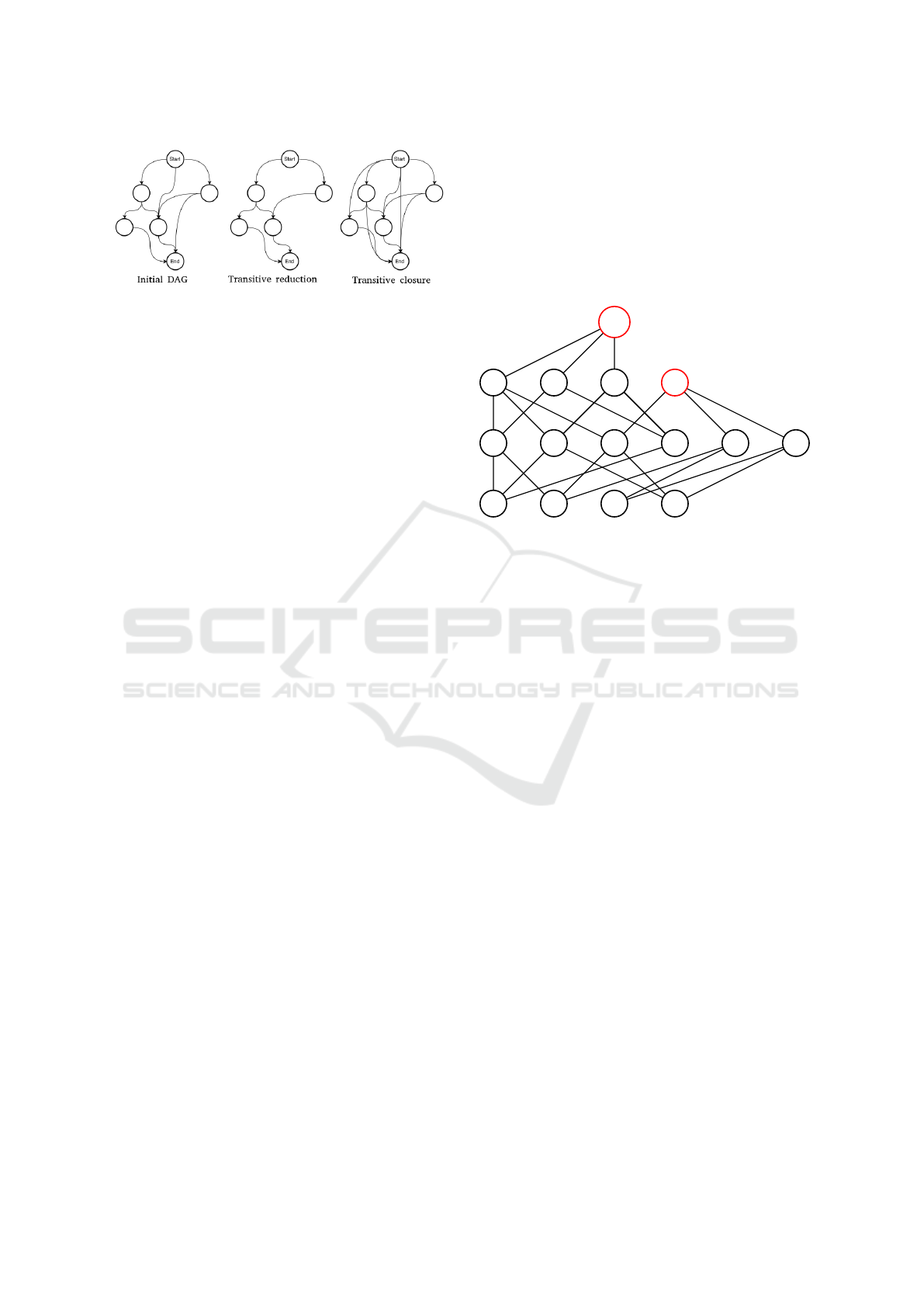
Figure 1: Transitive reduction / closure.
For sake of simplicity, in the rest of the article, an em-
bedding set is implicitly a Γ-embedding set. A max-
imal element of Γ is a sequence that is not a subse-
quence of any other elements of Γ.
Last, we use two common operators on graphs,
namely the transitive reduction (Aho et al., 1972) and
the transitive closure (Aho et al., 1972). The for-
mal definition of the transitive reduction of a directed
graph G is: A directed graph G’ is said to be a tran-
sitive reduction of the directed graph G provided that
G’ has a directed path from vertex u to vertex v, for
any (u,v), if and only if G has a directed path from
vertex u to vertex v, and there is no graph with fewer
arcs than G’ satisfying condition. The formal defini-
tion of the transitive closure of a directed graph G is:
A directed graph G’ is said to be a transitive closure
of the directed graph G provided that G’ has an edge
from vertex u to vertex v, for any (u,v), if and only if G
has a directed path from vertex u to vertex v. Figure 1
illustrates both operators, for directed acyclic graphs
(DAG) in our context.
3 THE EMBEDDING ANTICHAIN
We define the Embedding Antichain, noted A
Γ
, as the
Antichain that generates Γ.
Proposition 3.1. The Embedding Antichain is the
minimal set that represents all common subsequences
from n sequences.
Proof. A property of an Antichain is that it can gen-
erate a Lower Set of the subsequences of its elements.
As there is a one to one correspondence between an
Antichain and a Lower Set, the Embedding Antichain
is unique and is constituted by the maximal elements
of Γ. Hence, the Embedding Antichain is the minimal
set that represents all common subsequences from n
sequences. 
The representation of the Embedding Antichain
can be even more compact by constructing the min-
imal acyclic finite-state automata (AFSA) (Daciuk
et al., 2000) of this sequence set, because elements
Sn = { "abcdd",
"abddc" }
Gamma = { "a", "b", "c", "d", "ab", "ac",
"bc", "bd", "dd", "ad", "abc",
"bdd", "add", "abd", "abdd" }
A-Gamma = { "abc", "abdd" }
abcbddaddabd
abdd
ddab
ac
bc
bdad
a
b
c
d
A
Γ
Figure 2: A
Γ
representation.
of A
Γ
share symbols. It is a directed acyclic graph,
that has one root node (named START) and one leaf
node (named END). When enumerating all paths from
START to END, it generates A
Γ
. So our goal is to
build a minimal DAG that generates exactly A
Γ
. In
Figure 2, we show how A
Γ
represents Γ on a small
example.
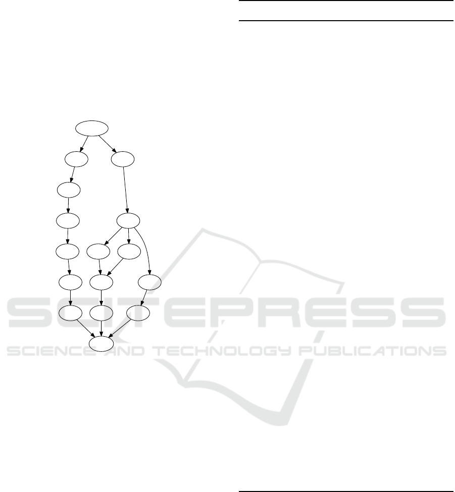
In Figure 3, we show an example of the construc-
tion of A
Γ
DAG from 4 more complex sequences. In
this example, enumerating all paths of the DAG from
START to END ends up generating A
Γ
. This DAG has
been generated by an implementation of the algorithm
we present in section 7.
We have identified that the number of intra-
sequence symbol repetitions — i.e. multiple occur-
rences of the same symbol in a sequence — is a factor
that has a very high impact on the branching factor
and the number of nodes of A
Γ
DAG. To get a bet-
ter understanding of the problem, we started solving
a problem with a reduced difficulty by adding a con-
straint on sequences: the case where each sequence
contains only unique symbols. We then expand the
solution found for the subproblem to build a solution
for the real problem. Throughout the article, we dis-
play instances of the algorithms on simple cases with
words. The sequences that we use on our real applica-
tion, and the output graph, cannot be displayed. They
are simply too large.
Systematic Characterization of a Sequence Group
647

Sn = { "absolumentsongeur",
"mensongeabsolu",
"solutionmensongere",
"songeusementresolue" }
A-Gamma = { "solu",
"sonso",
"soeso",
"mensoe" }
m
e
s
on
n e
l
s
s
u
o
o
END
e
START
Figure 3: Minimal A
Γ
DAG.
4 THE EMBEDDING ANTICHAIN
BETWEEN TWO SEQUENCES
WITHOUT INTRA-REPETIONS
As we show in the next parts, repeated symbols in a
sequence are an important contribution to the com-
plexity of the problem. Adding constraints to our
problem helps to compartment the different subprob-
lems.
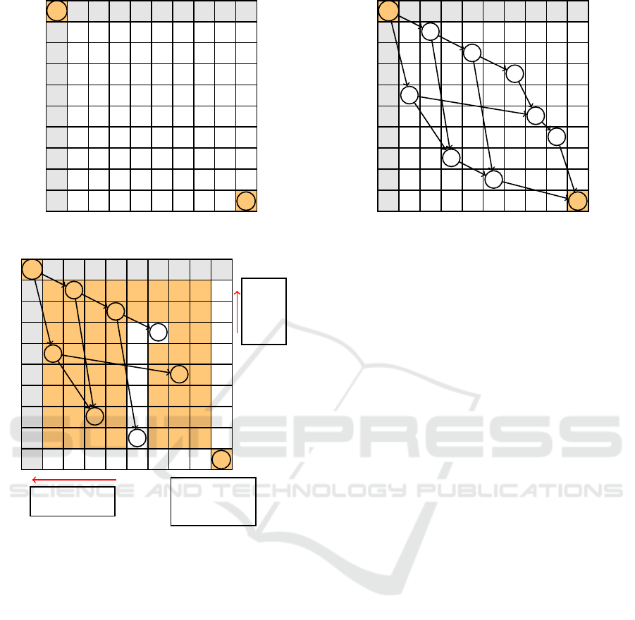
The following algorithm computes a DAG that
exactly produces A
Γ
when enumerating all possible
paths from the START node to the END node. Each
step is illustrated with an example, with the sequences
0
ABCDEFGH
0
and
0
BDFAGHCE
0
(Figures 4, 5 and
6):
Algorithm 1: A
Γ
for two sequences with no repeat.
input: s1 and s2, two sequences of size |s1|
and |s2|
output: G(V, A), a DAG
begin
create a matrix M of size (|s1|+2) * (|s2|+2)
fill M[0][0] with a node of value START
fill M[|s1|+1][|s2|+1] with a node of
value END
for 0 < i < |s1|
for 0 < j < |s2|
if s1[i] = s2[j]
fill M[i+1][j+1] with a node of
value s1[i]
else
fill M[i+1][j+1] with a node of
null value
end if
end for
end for
mark the node START as a node to process
while there are nodes to process
node <- take the first one on the list
mark all non null nodes in M as valid
mark all nodes in M with
i <= node.i and j <= node.j as invalid
L <- list elements in M
sort L in increasing order with the manhattan
distance between node and L elements
for element in L
if element is valid
add an edge linking node to element
mark all elements in M
with i >= element.i
and j >= element.j as invalid
add element as a node to process
end if
end for
end while
end
Proposition 4.1. Algorithm 1 produces the minimal
A
Γ
DAG.
Proof. The DAG nodes are common symbols and
they are connected in increasing index order — in-
creasing from both sequences. It produces Γ, the set
of all common subsequences, meaning that the DAG
produces a Γ-embedding set.
Moreover let us assume that the DAG does not
produce any antichain. Let us consider all the pos-
sible paths from START to END. The sequences have
ForSE 2019 - 3rd International Workshop on FORmal methods for Security Engineering
648

A B C D E F G H
B B
D D
F F
A A
G G
H H
C C
E E
Start
End
Figure 4: Initilization.
A B C D E F G H
B B
D D
F F
A A
G G
H H
C C
E E
Start
End
The next
node can-
not
come be-
fore
D in s
2
The next node can-
not come before D
in s
1
Once F is chosen,
the nodes after it
in s
1
& s
2
are be-
yond the scope of
the current iteration
Figure 5: Applying constraints on D for determining the
next nodes of the DAG (E and F). Colored boxed cannot be
chosen.
no intra-repetition, so each DAG symbol. It means
that at least one path of the graph is a subsequence
of one other path. It implies the following situation,
considering 3 arbitrary nodes A, B and C:
A -> B
B -> C
A -> C
If A is connected to B and C, it means that C is
not reachable from B because the algorithm connects
the current node to the closest one then constraints
the next connections to nodes that are not reachable
by the added child.
Consequently, this algorithm exactly produces the
DAG of A
Γ
for two sequences without repetition. As
no arc or node can be removed without contradicting
the previous properties, we also know that this is the
minimal DAG that produce A
Γ
. 
A B C D E F G H
B B
D D
F F
A A
G G
H H
C C
E E
Start
End
Figure 6: Building A
Γ
for two sequences without intra-
repetition.
5 THE EMBEDDING ANTICHAIN
OF N SEQUENCES WITHOUT
INTRA-REPETITION
The strategy we chose for finding the minimal A
Γ
DAG of more than two sequences is incremental. We
start with the previous algorithm for two sequences
to get an initial A
Γ
DAG. Then we process the se-
quences one after the other. We have found that this
problem we are solving is very similar to the problem
of building a minimal acyclic finite-state automata
(AFSA) (Daciuk et al., 2000) of a word set. In this do-
main, researchers also chose an incremental strategy.
Nonetheless, there are two major differences between
this problem and ours. On the first hand we cannot
represent or know in advance the elements of the word
set. In our problem the word set is the common sub-
sequence set, and as shown previously it grows expo-
nentially with the sizes of the sequences. As such, we
cannot represent it at any point of the solution. On
the other hand, our DAG must be a transitive reduc-
tion (Aho et al., 1972), meaning we cannot remove an
edge from the graph without removing a path from a
vertex v to a vertex w. Hence, any solution for build-
ing the AFSA in the litterature are of no help here.
Moreover, our graph yields more constraints than the
classical AFSA. The new DAG exhibits the following
properties:
• The DAG must be a transitive reduction otherwise
there would be a path that is a subsequence of one
other path.
• Each symbol is unique in the DAG because in
each sequence, symbols are unique.
• As we process new sequences, the graph cannot
grow in terms of vertices because symbols are
Systematic Characterization of a Sequence Group
649

unique.
• Let n be a node from the new DAG. Its children
cannot come before in the topological order of
the current DAG and in the indexes of the new se-
quence to process. These constraints hold because
symbols are unique both in the current DAG and
in the sequence to process.
• An edge cannot exist in the new DAG if this edge
is not in the transitive closure of the current DAG.
In other words, a node B is reachable from A in the
new DAG if B is reachable from A in the current
DAG.
The following algorithm computes the minimal
A
Γ
DAG and is illustrated with an example on
three sequences
0
ABCDEFGH
0
,
0
BDFAGHCE
0
and
0
EBGDFHAC
0
. The first and second sequences have
been processed by the algorithm from the previous
section to generate an initial DAG (Figure 7).
Algorithm 2: Minimal A
Γ
DAG of n + 1 sequences with no
repetition, from the minimal A
Γ
DAG of n sequences.
input: G(V, A) a DAG and s a sequence of size |s|
output: G’(V’, A’), a DAG
begin
Let ’depthMap’ be a map, that take as value a
list of nodes and as key their corresponding
depth in the DAG
depthMap <- topologicalSort( G(V, A) )
Let ’maxDepth’ be the maximum key of depthMap
Let ’TC’ be the transitive closure matrix of
G(V, A) (size |V|*|V|)
mark the node START as a node to process
while there are nodes to process
node <- take the first one on the list
for element in M
if element.i > node.i
and element.j > node.j
and element is reachable from node in TC
add an edge linking node to element
end if
end for
end while
G’(V’, E’) <- transitiveReduction(G(V, E))
end
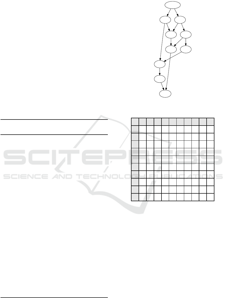
The Figure 10 presents the result on the three se-
quences example.
START
A B
END
C
G
D
E
H
F
Figure 7: Starting A
Γ
DAG (result from previous section).
A B C D E F G H
0 1 1 1 1 1 1 1 1 1
A 0 0 0 1 0 1 0 1 1 1
B 0 0 0 1 1 1 1 1 1 1
C 0 0 0 0 0 1 0 0 0 1
D 0 0 0 0 0 1 1 1 0 1
E 0 0 0 0 0 0 0 0 0 1
F 0 0 0 0 0 0 0 1 1 1
G 0 0 0 0 0 0 0 0 1 1
H 0 0 0 0 0 0 0 0 0 1
0 0 0 0 0 0 0 0 0 1
Start
Start
End
End
Figure 8: Transitive closure of G(V, A) (’TC’).
Proposition 5.1. Algorithm 10 produces the minimal
A
Γ
DAG.
Proof. The algorithm starts essentially to connect all
nodes to all other, excluding the impossible cases:
• A node cannot connect to a node that has a lower
or equal topological order.
• A node cannot connect to a node that has a lower
or equal sequence index.
• A node cannot connect to a node that is not reach-
able in the transitive closure.
These three conditions of node connections cannot
remove a common subsequence. As a consequence,
by enumerating all paths from START to END, it gen-
erates all possible common subsequences. At this
point the DAG is already Γ-embedding. Then, by
ForSE 2019 - 3rd International Workshop on FORmal methods for Security Engineering
650

E B G D F H A C
0
1 B A
2 D C
3 E F
4 G
5 H
6
Start
End
Start
End
Figure 9: New DAG initialization.
START
A B
E
END
C D
GF
H
Figure 10: Minimal A
Γ
DAG for three sequences.
applying the transitive reduction, the graph become
the minimal A
Γ
DAG because symbols are unique so
there cannot be two equal paths in the DAG. As nodes
have unique symbols, no edge can be removed from
the transitive reduction of the DAG without remov-
ing a subsequence. Therefore the graph is minimal
and its paths form an antichain. It is the minimal A
Γ
DAG. 
6 THE EMBEDDING ANTICHAIN
OF TWO SEQUENCES
The intra-sequence symbol repetition invalidates the
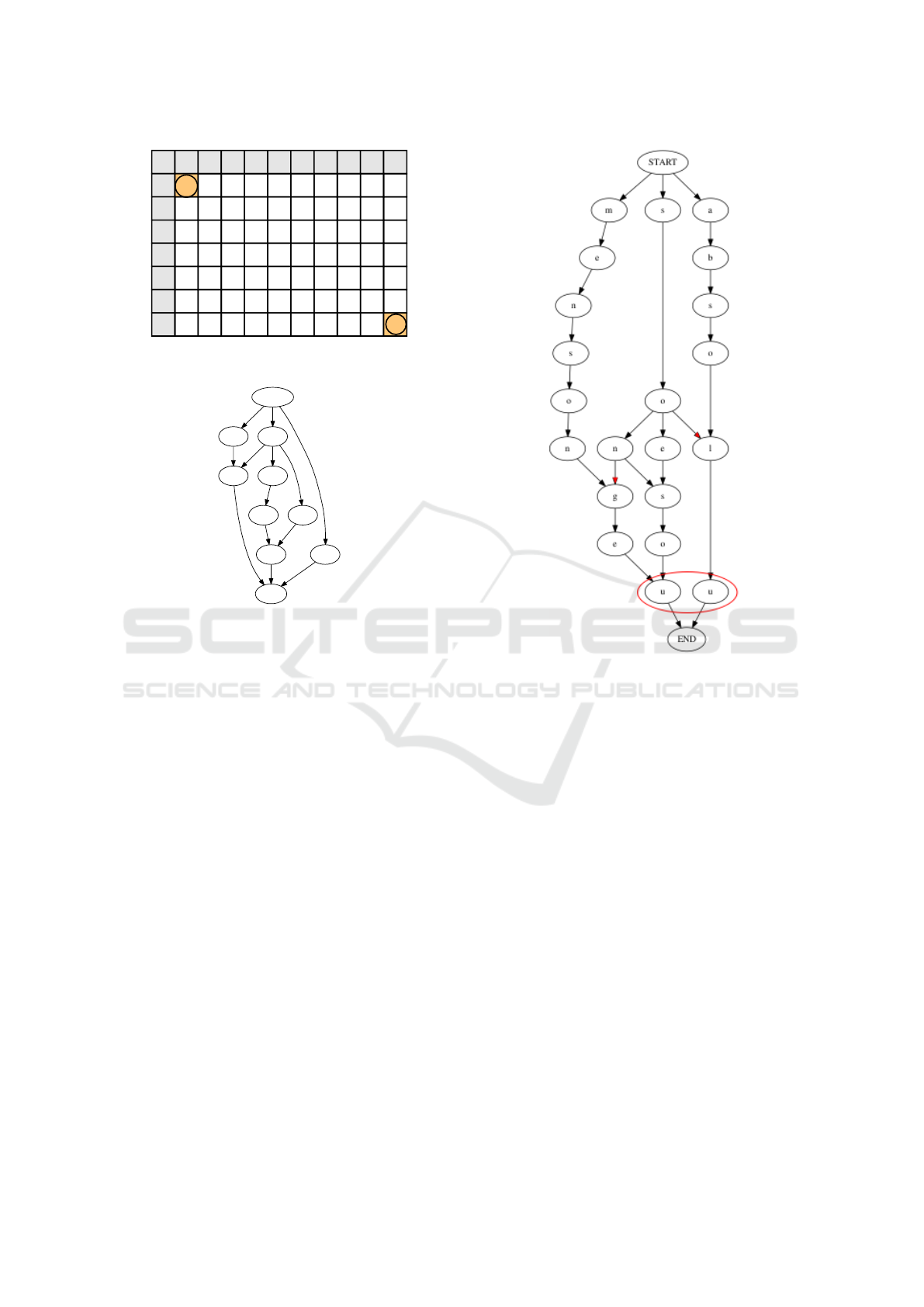
proof of the algorithm 1. To understand what sym-
bol repetition induces, we applied the algorithm 1 on
this new problem. We choose the sequences ”absolu-
mentsongeur” and ”mensongeabsolu” (Figure 11) to
illustrate the problematic.
The objective is to produce a minimal A
Γ
DAG.
We note that the DAG does not represent an antichain,
we have highlighted in Figure 11 two edges that pro-
duces sequences that are subsequences of longer paths
from START to END. The DAG is also not minimal
Figure 11: Algorithm 1 on two sequences with intra-
repetitions.
because we can merge the two nodes ’u’ while being
able to produce the exactly same unique paths. How-
ever the DAG produces a Γ-embedding set. The DAG
nodes are common symbols and they are connected
in increasing index order — increasing from both se-
quences. It means that the DAG always produces a
Γ-embedding set.
We can easily make the DAG minimal by merging
equivalent nodes at the end of the algorithm 1. Equiv-
alent nodes are nodes with equal symbols that have
exactly the same children or parents. When equivalent
nodes are merged, a new node is created with children
and parents from both equivalent nodes. However, de-
signing an algorithm for finding the supernumerary
edges (marked in red in Figure 11) is a challenging
task regarding the fact that path enumeration in the
graph has a polynomial complexity of high order.
Proposition 6.1. The worst case complexity of path
enumeration of a minimal Γ-embedding DAG is
O(n
k+1
) where n is the maximal number of nodes from
all topological levels and k is the number of topolog-
ical levels.
Systematic Characterization of a Sequence Group
651

Proof. We construct a DAG, denoted B, that con-
tains all the sequences from a minimal Γ-embedding
DAG, denoted A. This DAG has n ∗ k, n nodes in
each topological level. The nodes from A are in B
in the same topological levels. All nodes are con-
nected to all nodes from its next topological level. B
has n
k+1
paths, so the worst case complexity of A is
O(n
k+1
). 
For the computation of the minimal A
Γ
DAG, we
tried different methods. None of them can compute
the minimal A
Γ
DAG with an acceptable algorithmic
complexity. Our best attempt is founded on the fact
that with reversed sequences for each DAG node, its
children should be its parents and conversely. We note
that applying 1 in forward and backward order leads
to different DAG that are not equivalent when revers-
ing children and parents. Relying on this observation,
we reached an algorithm close to the solution:
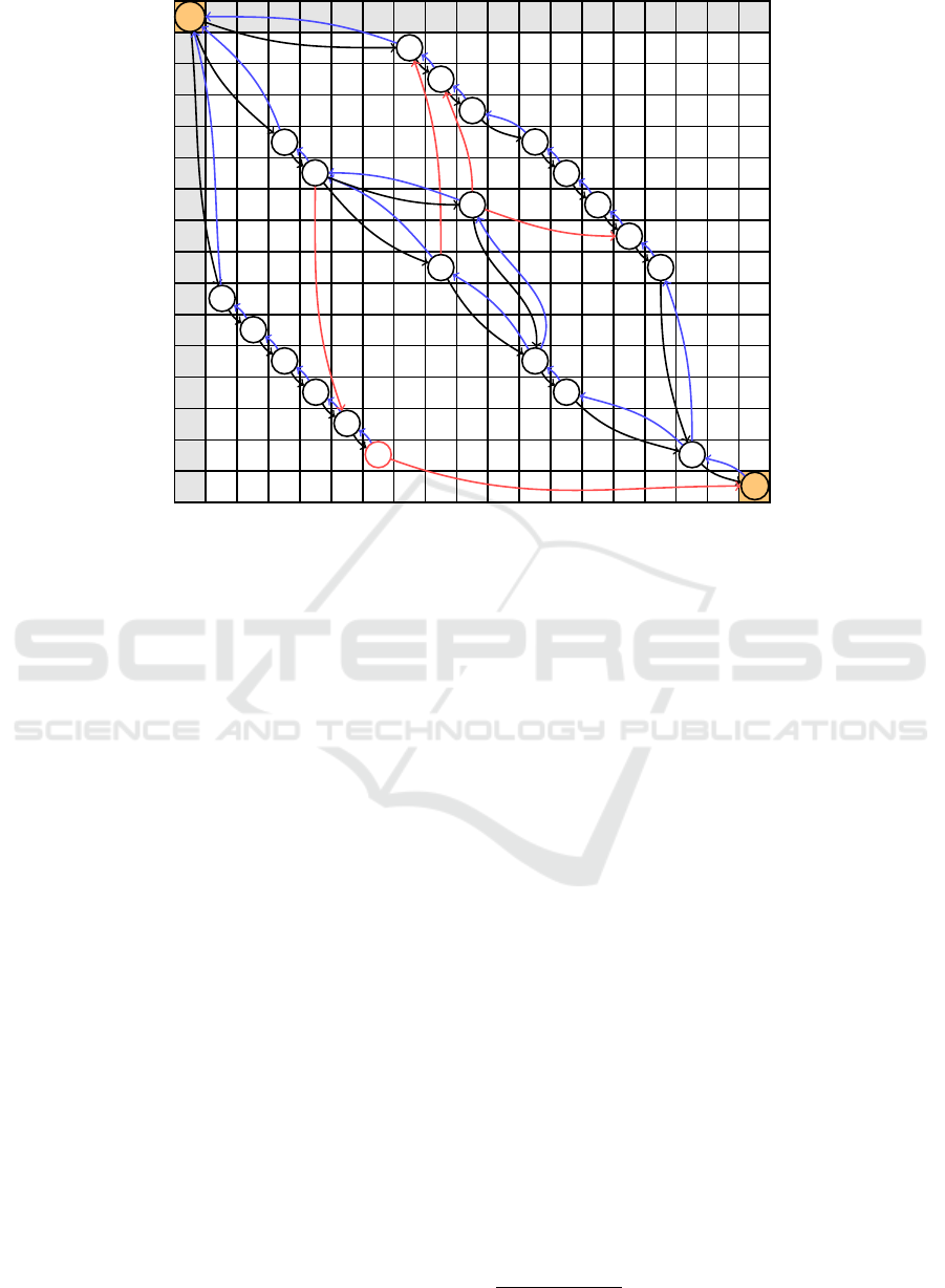
Algorithm 3: Subsequence DAG for two sequences.
1. Apply algorithm 1 from Start to End (forward pass) and from
End to Start (backward pass). The backward pass is the equiv-
alent to a forward pass with sequences in reverse order.
2. Merge equivalent vertices. Equivalent vertices are two vertices
that have the same symbols and the same children or the same
parents. Edges from the forward and backward passes are con-
sidered for the children/parent comparison. If no nodes have
been merged, go to step 5.
3. Apply the transitive reduction on both forward and backward
graphs. If no edge has been deleted, go to step 5.
4. Go to step 2.
5. Delete all edges that have no equivalent edge in the other pass.
An edge from vertex v to u from the forward pass is considered
equivalent to an edge from u to v from the backward pass.
6. Some nodes can be left without parents, we call them orphan
nodes. Link the orphan nodes to its parents in the forward and
the backward DAG that have a common symbol and that still
exists in the current DAG. If no such parent has been found,
delete the orphan node.
7. Some nodes can be left without children, we call them single
nodes. Link the single nodes to its children in the forward and
the backward DAG that have a common symbol and that still
exists in the current DAG. If no such child has been found,
delete the single node.
8. If an orphan or single node has been deleted, go to step 6.
This algorithm works on the example with ”ab-
solumentsongeur” and ”mensongeabsolu”, as shown
in Figure 12.
However, when tested with longer sequences we
noted that this additional constraint on the edges in-
duces a problem and we found that this algorithm
does not produce A
Γ
or a Γ-embedding set, but a set
that contains less or equal information. This problem
arises when a forward path is equivalent to a back-
ward pass but with different nodes.
7 THE EMBEDDING ANTICHAIN
OF N SEQUENCES
Compared to the same problem without intra-
repetition, processing the Γ-embedding DAG of n +
1 sequences from the Γ-embedding DAG of n se-
quences brings two new difficulties. The first one
is that each node from the previous DAG, that have
several matches in the new sequence, must be dupli-
cated in the {topological level / sequence index} ma-
trix. It means, when using the algorithm 4 for an ar-
bitrary node, that it can connect to children that are
duplicated, actually creating duplicated paths or su-
pernunary subsequences. To cope with this problem,
a node must not be connected to more than one dupli-
cated child. The second problem is the introduction
of duplicated paths as two different nodes can have
the same symbols. Like in the previous section, we
apply a {merge / transitive} reduction phase to re-
move the most part of it. If the previous graph is a
Γ-embedding DAG of n + 1 sequences then the result
is a Γ-embedding DAG, because none of the steps can
remove a node or an edge that breeds a unique subse-
quence. Here is the full algorithm:
Algorithm 4: Γ-embedding DAG for n+1 sequences from a
Γ-embedding DAG of n sequences.
1. Process a topological sort and the transitive closure of the
DAG.
2. For each node in the DAG create a new node for each corre-
sponding symbol in the sequence. Every new node created at
one iteration is called duplicated node.
3. Connect each new node, of topological level i and of sequence
index j, to all new nodes that satisfy the following conditions:
• It comes from a node reachable in the transitive closure of
the DAG.
• Its topological level is at minimum i + 1.
• Its sequence index is at minimum j + 1.
• The node has not been connected to another duplicated
node.
4. Merge equivalent vertices. Equivalent vertices are two vertices
that have the same symbol and the same children or the same
parents. If it is not the first iteration of the merge phase and no
vertex have been merged, stop the algorithm.
5. Process the transitive reduction of the current graph. If no edge
has been deleted, stop the algorithm.
6. Go to step 4.
ForSE 2019 - 3rd International Workshop on FORmal methods for Security Engineering
652

A B S O L U M E N T S O N G E U R
M M
E E
1
E
N N
1
N
S S
1
S
3
O O
1
O
3
N N
3
N
2
G G
E E
3
E
2
A A
B B
S S
2
S
4
O O
2
O
4
L L
U U U
Start
End
Figure 12: Applying algorithm 1 forward and backward.
−− >: Forward pass Vertex: Vertex to merge
< −−: Backward pass < − − / − − >: Path to delete
8 EXPERIMENTAL RESULTS
In this part, we test our final algorithm on sequences
coming from the dynamic analysis of benign and mal-
ware applications. In a first part, we explain how we
gather and process the sequences from Android appli-
cations. In a second part, we explore a way of using
the graph produced by our algorithm to detect if an
application belongs to a particular malware family
8.1 Sequence Collection and Processing
We use a dataset of 719 Android malware and 521
benign samples. Malware samples come from the
Drebin Dataset (Arp et al., 2014). It is the most
widely used malware dataset, in the domain of An-
droid malware detection. In a previous study (Irolla
and Dey, 2018), we observed that a large part of mal-
ware samples from this dataset share the same opcode
sequences — i.e. the bytecode sequence without the
operand. A large part of malware applications use
repackaging, this is why for two malware samples that
share the same opcode sequence, the only changes are
often strings, class names and assets. 49.35% of ap-
plications have this characteristic. We showed that it
artificially boost the performance of machine learning
algorithms because samples that have been learned
from the training set are also found in the testing set.
So, in our experiment we only use malware samples
that exhibit different opcode sequences, that way we
get an unbiased performance result of generalization
capacity of the algorithm. The benign samples come
from F-Droid
1
, a repository of Free and Open Source
Android applications. These applications cannot a
priori be malicious.
We chose to represent a sample by the sequence
of Java calls to the Android API it executes during a
dynamic analysis process. The Java call sequence is
used to model the behavior of the application. It is an
information used in the detection of malware, recov-
ered mainly through static analysis. Java calls can be
methods implemented by the developer — which then
have a prior unknown behavior — or methods imple-
mented in external libraries. The Android API is of-
ten the only entry point for accessing certain phone
features. Information that identifies the phone or the
user, access to SMS, calls, contacts, etc. Using these
calls to the Android API in an unusual way may re-
veal mischievous behavior. Researchers have already
studied the usage of these API call sequences to the
malware detection problem. DroidAPIminer (Aafer
et al., 2013) achieve 99% accuracy with KNN (Aha
et al., 1991), on a dataset of 3987 malware samples
and 500 benign samples with split testing (66% learn-
1
https://f-droid.org
Systematic Characterization of a Sequence Group
653

Figure 13: Tandem repeat removal algorithm.
ing, 33% testing). Feng Shen et al. (Shen et al., 2018)
achieve 94.5% accuracy with a SVM classifier on a
dataset of 3899 malware samples, 3899 benign sam-
ples with split validation (90% learning, 10% testing).
It appears that API calls are also a feature with potent
discriminative power.
The whole system that tests, executes applications
and collects Java calls is Glassbox (Irolla and Filiol,
2017). The application UI relies on pooling loops to
be reactive, and a large portion of the code logic is
handled by loops. This results in repeated substrings
within the sequence. These repeated substrings do not
convey new information and hinders both the perfor-
mance and efficiency of algorithms that process them.
These artefacts, in the domain of biology are called
tandem repeat
2
. Lin & al. (Lin et al., 2015) also
identified this problem in their study of system call
sequences from the dynamic analysis of applications.
They solved it by removing consecutive call repeti-
tion, i.e. tandem repeats of size 1. We designed a tan-
dem repeat removal algorithm to increase both perfor-
mance and efficiency of downstream algorithms. Let
be ttr, a function that keep only the first instance of
every tandem repeat. For example:
trr(”aezezezabcdabcd”) = ”aezabcd”
The algorithm we use is inspired from a naive ap-
proach. In Figure 13 we show this algorithm running
on the previous example.
On the diagonal is the number of the iteration. To
detect a tandem repeat, we run the matrix, noted m,
downwards, starting from the current iteration on the
diagonal, until we find a position where m(i, j) = 1.
The distance d, between the starting point and the
first valid position is saved. Then, we run the ma-
trix diagonally until a non-valid position is found, i.e.
m(i, j) = 0. We save the traveled distance, d
0
. We
have d
0
= k.d + r with (k, r) ∈ N
2
. Last we erase the
2
https://meshb.nlm.nih.gov/record/ui?ui=D020080
k.d first positions from the diagonal. To erase a po-
sition (i, j), we remove all (i
0
, j) and all ( j, i
0
) for all
i
0
possible positions. Then the matrix is reassembled.
In our example, removal appeared at iteration 2 and 4.
This naive algorithm is obviously of O(n
2
) time
and space complexity where n is the sequence size.
It is impractical. We noted that tandem repeat size in
our data rarely exceed 10. So we break the sequence
in parts of random size — between 100 and 500 —
and apply this algorithm on them. As the breaks can
happen in the middle of a tandem repeat, we apply
again this procedure until there is no change in the se-
quence or 3 times maximum. In this way, our tandem
repeat removal algorithm becomes O(n) in time and
space complexity.
8.2 Classification Experiment
The Γ-embedding DAG contains common informa-
tion between a group of sequences. To exploit these
data for assessing if a new sequence belongs or not
to the group, we need to define measures. Let us de-
tail our approach. We collect common symbols be-
tween all sequences from a group, then we remove
any non-common symbols from all sequences. These
sequences are sorted by their length in increasing or-
der. It becomes the order of sequence processing.
As the shortest sequences are treated first, it is most
likely that at each iteration, we get the smaller possi-
ble DAG.
We apply the algorithm 3 on the two first se-
quences and the algorithm 4 for the following ones.
To assess if a new sequence belongs to the group,
we use the algorithm 4 again with the DAG from the
group. Then we define several measures that give in-
dications about the changes on the DAG. The less the
DAG is reduced, the most likely the new sequence be-
longs to the group because it shares a wide number of
common subsequences.
Let N
b
,E
b
,P
b
be respectively the number of nodes,
edges and paths (from START to END) in the DAG
before the new sequence processing. Let N
a
,E
a
,P
a
be respectively the number of nodes, edges and paths
in the DAG after the new sequence processing. We
define three criteria: node expansion, edge expansion
and path expansion noted N
ex
,E
ex
and P
ex
.
N
ex
=
N
a
− N
b
N
b
,E
ex
=
E
a
− E
b
E
b
,P
ex
=
P
a
− P
b
P
b
Algorithm 4 is very sensitive to outliers in se-
quence clusters. The sequence that share the less
common subsequences with the group will reduce the
graph the most. For that reason, we re-clustered mal-
ware families to get groups of sequences that are re-
ForSE 2019 - 3rd International Workshop on FORmal methods for Security Engineering
654

ally close. To accomplish this task, we use a dis-
tance between two sequence clusters that favor com-
mon subsequences:
D(c
1
,c
2
) =
1
|A
c
1
∩ A
c
2
|
, the inter-cluster distance
D(c,c) =
1
|A
c
|
, the intra-cluster distance
Where A
c
is the set of symbols in the sequence cluster
c. 0 < D(c
1
,c
2
) ≤ 1. When the sequences in a group
share a lot a common symbols, D tends to 0, and con-
versely when the sequences share just a few symbols,
D tends to 1.
We have designed a hierarchical clustering to
group similar sequences based on the D distance.
At initialization, each sequence is within a separated
cluster, then at each iteration, the clusters that have
the lowest distance are merged. The common sym-
bols between both clusters become the symbol set of
the new cluster. In that sense, when clusters are cre-
ated we lose the information about the individual se-
quences. To find the optimal number of cluster we
minimize a Ward criterion:
r =
∑
∀c
i
∈C
D(c
i
,c
i
)
2
∑
∀c
i
,c
j
∈C∗C|i6= j
D(c
i
,c
j
)
2
Where C is the set of clusters. At each iteration r is
calculated and the iteration with the lowest r is con-
sidered as the optimal iteration. To promote clusters
that are consistent regarding our problem, we added
several constrains to the clusters:
• At least 50% of the points must be clustered
• Clusters of size 1 are not considered (even in r
calculation)
• Clusters of size below 20% of the maximal size
among clusters are not considered (even in r cal-
culation).
These rules ensure that small clusters are filtered
— they are outliers regarding our problem — and that
at least a majority of the malware dataset is taken into
account. Another issue is that Android malware and
benign applications share API patterns linked to the
use of UI. The common subsequences derived from
UI API calls is of little use on malware detection.
Hence, to refine malware sequences, we first cluster
benign applications, take the symbols sets of the valid
clusters and subtract them from malware sequences
(Table 2).
Then we cluster malware sequences, results are
presented in Table 3.
Table 1: Topological sort of G(V, A) (’depthMap’).
Order 0 1 2 3 4 5 6
Vertices START A,B C,D E,F G H END
Table 2: Benign sequence clusters.
Cluster N
o
number of sequences number of common symbols
0 15 289
1 8 33
2 16 23
3 9 21
Table 3: Malware sequence clusters.
Cluster N
o
number of sequences number of common symbols
0 15 34
1 28 20
2 33 75
3 11 23
4 22 17
5 12 39
Table 4: Leave-one-out cross validation measures.
Cluster N
o
0 1 4
Node expansion mean 0% -2.455% -2.769%
Node expansion standard deviation 0% 7.411% 12.262%
Edge expansion mean 0% -2.469% -2.702%
Edge expansion standard deviation 0% 7.673% 12.013%
Path expansion mean 0% 0% -1.705%
Path expansion standard deviation 0% 0% 7.995%
We note that benign sequences are more diverse —
48 / 521 benign sequences within selected clusters
— than malware sequences — 121 / 719 malware
sequences within selected clusters. We use only
malware clusters 0, 1 and 4 because they lead to
Γ-embedding DAG that are very fast to generate.
Other clusters lead to DAGs with more than 10
5
nodes
and edges. They require too much computing time
to generate. The approximation we get lead to er-
rors, mostly added nodes and edges. These errors
grow with the number and size of the common sub-
sequences. For some pathological cases, the graph is
constitued mostly by errors. So, before the graph is
reduced by the node merging and transitive reduction
phases, the intermediate graphs are already too big to
be processed. A better approximation should enable
more cases to be processed. This subject still requires
extensive research, as it is a domain at its beginning.
Next, for each cluster we use leave-one-out cross
validation. One sequence is removed from a clus-
ter, then the Γ-embedding DAG is processed from the
rest. The sequence that has been left out is added to
the DAG and we measure the node, edge and path ex-
pansion, the results are presented in Table 4.
The standard deviation of {node, edge, path} ex-
pansion is used as a criterion of a sequence belonging
to a cluster. We consider that a new sequence belongs
a cluster if its {node, edge and path} expansion devi-
ation from the mean is below the respective standard
Systematic Characterization of a Sequence Group
655

Table 5: Classification results.
Correct classification
leave-one-out malware clusters 59 / 65 (90.77%)
malware sequences 654 / 654 (100%)
benign sequences 499 / 521 (95.77%)
overall 1212 / 1240 (97.74%)
deviations. We tested all benign sequences and all
malware sequences — that were not already belong-
ing to a cluster. The results are presented in Table 5.
A sequence is considered to be correctly classified
if a sequence is predicted to belong in the right clus-
ter for leave-one-out malware sequences or if the se-
quence is predicted to not belong to any of the clusters
for the rest of the sequences. The overall results of
97.74% accuracy is close to the state-of-the-art (98%
(Deshotels et al., 2014), 99% (Aafer et al., 2013),
97.3-99% (Yerima et al., 2015)). The limitation is that
we could not make consistent Γ-embedding DAG for
the whole dataset. The process of DAG creation or
clustering needs improvement to enable a larger us-
age of the Γ-embedding DAG. However it shows that
this mathematical object (Γ-embedding DAG) is use-
ful for production applications.
9 CONCLUSION
This article contributes to the state-of-the-art by defin-
ing, formalizing and constructing a new representa-
tion for the common subsequences of a sequence set.
It is called A
Γ
DAG. We showed that the A
Γ
DAG con-
tains all information about the common subsequences
and is expressed in a very compact form. We succeed
to design an algorithm that is able to build this con-
struction for sequence without intra-repetitions. For
other sequences, we have designed an algorithm that
is able to construct a structure close to solution.
We assessed its utility for classification heuristics.
With simple metrics we came to 97.74% accuracy for
singling out clustered malware from other applica-
tions with the sequence of their Android API calls ex-
ecuted during dynamic analysis. While it does com-
pete with state-of-the-art malware detection with ma-
chine learning, it shows that Γ-embedding DAG con-
veys enough information for classification. The ex-
ploitation of this representation for data mining needs
further researches.
REFERENCES
Aafer, Y., Du, W., and Yin, H. (2013). Droidapiminer:
Mining api-level features for robust malware detection
in android. pages 86–103. DOI 10.1007/978-3-319-
04283-1 6.
Aha, D. W., Kibler, D., and Albert, M. K. (1991).
Instance-based learning algorithms. Machine learn-
ing, 6(1):37–66.
Aho, A. V., Garey, M. R., and Ullman, J. D.
(1972). The transitive reduction of a directed graph.
SIAM Journal on Computing, 1(2):131–137. DOI
10.7146/math.scand.a-10849.
Arp, D., Spreitzenbarth, M., Hubner, M., Gascon, H.,
Rieck, K., and Siemens, C. (2014). Drebin: Effective
and explainable detection of android malware in your
pocket. 14:23–26. DOI 10.14722/ndss.2014.23247.
Cheatham, M. and Hitzler, P. (2013). String similarity met-
rics for ontology alignment. pages 294–309.
Daciuk, J., Mihov, S., Watson, B. W., and Watson,
R. E. (2000). Incremental construction of minimal
acyclic finite-state automata. Computational linguis-
tics, 26(1):3–16. DOI 10.3115/1611533.1611538.
D’Angelo, J. P. and West, D. B. (2000). Mathemati-
cal Thinking: Problem-Solving and Proofs, 2nd ed.
Prentice-Hall. DOI 10.4324/9781315044613.
Deshotels, L., Notani, V., and Lakhotia, A. (2014). Droi-
dlegacy: Automated familial classification of android
malware. page 3. DOI 10.1145/2556464.2556467.
Hirschberg, D. S. (1975). A linear space algorithm for
computing maximal common subsequences. Com-
munications of the ACM, 18(6):341–343. DOI
10.1145/360825.360861.
Irolla, P. and Dey, A. (2018). The duplication issue within
the drebin dataset. Journal of Computer Virology and
Hacking Techniques, pages 1–5.
Irolla, P. and Filiol, E. (2017). Glassbox: Dynamic analy-
sis platform for malware android applications on real
devices. ForSE. DOI 10.5220/0006094006100621.
Lin, Y.-D., Lai, Y.-C., Lu, C.-N., Hsu, P.-K., and Lee, C.-
Y. (2015). Three-phase behavior-based detection and
classification of known and unknown malware. Secu-
rity and Communication Networks, 8(11):2004–2015.
DOI 10.1002/sec.1148.
Mount, D. W. Bioinformatics: sequence and genome anal-
ysis. 2004. Bioinformatics: Sequence and Genome
Analysis.
Shen, F., Del Vecchio, J., Mohaisen, A., Ko, S., and Ziarek,
L. (2018). Android malware detection using complex-
flows. IEEE Transactions on Mobile Computing.
Yerima, S. Y., Sezer, S., and Muttik, I. (2015). High accu-
racy android malware detection using ensemble learn-
ing. IET Information Security, 9(6):313–320. DOI
10.1049/iet-ifs.2014.0099.
ForSE 2019 - 3rd International Workshop on FORmal methods for Security Engineering
656