Deep Learning-based Method for Classifying and Localizing Potato
Blemishes
Sofia Marino, Pierre Beauseroy and André Smolarz
Institut Charles Delaunay/M2S, FRE 2019, Université de Technologie de Troyes,
Keywords:
Deep Learning, Potato Blemishes, Classification, Localization, Autoencoder, SVM.
Abstract:
In this paper we address the problem of potato blemish classification and localization. A large database with
multiple varieties was created containing 6 classes, i.e., healthy, damaged, greening, black dot, common scab
and black scurf. A Convolutional Neural Network was trained to classify face potato images and was also
used as a filter to select faces where more analysis was required. Then, a combination of autoencoder and
SVMs was applied on the selected images to detect damaged and greening defects in a patch-wise manner.
The localization results were used to classify the potato according to the severity of the blemish. A final
global evaluation of the potato was done where four face images per potato were considered to characterize
the entire tuber. Experimental results show a face-wise average precision of 95% and average recall of 93%.
For damaged and greening patch-wise localization, we achieve a False Positive Rate of 4.2% and 5.5% and
a False Negative Rate of 14.2% and 28.1% respectively. Concerning the final potato-wise classification, we
achieved in a test dataset an average precision of 92% and average recall of 91%.
1 INTRODUCTION
Potato is one of the most important food crops con-
sumed all over the world with a total production that
exceeds 374.000.000 tons (IPC, 2018). The physi-
cal aspect of this edible tuber is of great importance
in determining the market price between the diffe-
rent stages of the supply chain. Their quality is af-
fected by different types of blemishes that may be
visually identified. In most cases, the quality cont-
rol is still done manually by human operators, where
the main drawbacks are: subjectivity and high labor
costs. Thus, several inspection methods have been
developed to automate these tasks in a more efficient
and cost-effective way. Computer vision and machine
learning techniques have been applied successfully
in the quality control of agricultural produce (Barnes
et al., 2010; Jhuria et al., 2013; Zaborowicz et al.,
2017). The first works were focused on computer
vision systems consisted of three main stages: fir-
stly, pre-processing of images acquired by cameras
were done. Secondly, hand-crafted features were ex-
tracted in order to obtain relevant information about
the object and finally, machine learning techniques
were used to classify according to features extracted
(Miller and Delwiche, 1989; Bolle et al., 1996; Tao
et al., 1995). The key problem with these systems
is the difficulty to design a feature extractor adap-
ted to each pattern, that require human expertise to
suitable transform the raw input image into a good
representation, exploitable to achieve the classifica-
tion task. In the last few years, deep learning techni-
ques have demonstrated outstanding results in many
research fields, such as image classification (Mohanty
et al., 2016; Oppenheim and Shani, 2017; Picon et al.,
2018), object detection (Redmon et al., 2016), speech
recognition (Hinton et al., 2012) and semantic seg-
mentation (Badrinarayanan et al., 2015). The main
advantage of deep learning methods is their ability to
use raw data and automatically find the representa-
tion needed to achieve the classification or detection
task. Deep Learning applied in agriculture is gro-
wing rapidly with promising results (Mohanty et al.,
2016; Brahimi et al., 2017; Oppenheim and Shani,
2017). Unfortunately, these methods mainly use a
pixel-labeled dataset which construction is laborious
and time-consuming. For the remaining methods,
either they do not do blemish localization, i.e. they
do only classification, or an approximate localization
using a patch scale too large. Furthermore, deep le-
arning based methods are not widely explored in po-
tato blemish detection. The main contributions of this
work are as follows:
Marino, S., Beauseroy, P. and Smolarz, A.
Deep Learning-based Method for Classifying and Localizing Potato Blemishes.
DOI: 10.5220/0007350101070117
In Proceedings of the 8th International Conference on Pattern Recognition Applications and Methods (ICPRAM 2019), pages 107-117
ISBN: 978-989-758-351-3
Copyright
c
 2019 by SCITEPRESS – Science and Technology Publications, Lda. All rights reserved
107

• A large image-level labeled dataset that contains
6 different classes was created with the help of
two experts including multiple varieties of pota-
toes and images taken using multiple camera de-
vices.
• The created dataset was used to train an efficient
Convolutional Neural Network, that classifies po-
tato faces and also selects the images that require
further analysis.
• A combination of autoencoder and SVMs is pro-
posed to localize the damaged and greening areas
in these selected images.
• We introduced a global evaluation of the tuber ac-
cording to the previous results.
The paper is organized as follows: Section 2 presents
a brief related work. We detail our proposed method
in Section 3. Discussion and results are presented in
Section 4. Finally, we conclude the paper in Section
5.
2 RELATED WORK
Machine vision systems have been widely applied
to classification and blemish detection in agricultu-
ral produce. In (Bolle et al., 1996) authors propo-
sed a system to classify fruits and vegetables in gro-
cery and supermarkets stores. Color and texture his-
tograms were used as input to a nearest-neighbour
classifier achieving over 95% top-4 choices correct
responses. A vectorial normalization was proposed
in (Vízhányó and Felföldi, 2000) to differentiate bet-
ween the natural browning and the browning caused
by disease in mushrooms. In (Xing et al., 2005), a
method that use principal component analysis on hy-
perspectral images for determining apples as sound
or bruised was presented. An accuracy of about 93%
for detecting sound apples and 86% for bruised ap-
ples was achieved. In (Blasco et al., 2007), the aut-
hors introduced a region-oriented segmentation algo-
rithm to identify defects of citrus fruits. An accuracy
of 95% was obtained. A main drawback of this met-
hod is that authors assumed that most surface of the
fruit was of sound peel, which is not always the case.
A banana segmentation method was proposed in (Hu
et al., 2014). The segmentation of the banana from
the background and the detection of damaged lesi-
ons were made by two k-means clustering algorithms.
Machine vision systems applied to potatoes were stu-
died in several works. Authors in (Zhou et al., 1998)
applied color thresholding in HSV color space to de-
tect greening potatoes. In order to classify potatoes
by shape, they compared the detected potato boun-
dary with an ellipse which represented a good potato
shape. The projected area of the potato and the minor
axis of the fitted ellipse were also used for classifying
by weight and size respectively. The overall success
rate was 86.5%. In (Noordam et al., 2000), a method
for grading potatoes by size, shape and various de-
fects was introduced. Color and shape features were
used to train a Linear Discriminant Analysis combi-
ned with Mahalanobis distance classifier. Eccentri-
city and central moments were used to differentiate
between defects and diseases. Then, Fourier Descrip-
tors were used to detect misshapen potatoes. Unfor-
tunately, pixel-level labeled datasets were needed to
train and validate the models for each potato culti-
var. Potato classification in good, rotten and green
was presented in (Dacal-Nieto et al., 2009). Features
for every RGB and HSV channel were extracted using
histograms and co-occurrence matrices. Then, feature
selection was applied using a genetic algorithm to fi-
nally classify potatoes with a nearest neighbor algo-
rithm. Detection rate of 83.3%, 88.5% and 84.7% was
achieved for good, rotten and green potatoes respecti-
vely. (Barnes et al., 2010) introduced an AdaBoost
based system to discriminate between blemished and
non-blemish pixels. Color and texture features were
extracted and the best features for the classification
task were automatically selected by the AdaBoost al-
gorithm. They achieved a success rate of 89.6% for
white potatoes and 89.5% for red potatoes. Authors
in (ElMasry et al., 2012) developed a real-time system
to detect irregular potatoes. Geometrical features and
Fourier Descriptors were used as input to a Linear
Discriminant Analysis to identify the most relevant
features that were useful to characterize regular pota-
toes. A success rate of 98.8% for regular potatoes and
75% for misshapen potatoes was achieved in a test
experiment. A method based on Principal Compo-
nent Analysis combined with one-vs-one SVM multi-
classifier was proposed in (Xiong et al., 2017). They
attained an overall recognition rate of 96.6% for clas-
sifying potatoes in normal, green, germinated and da-
maged. Recently, various methods based on deep le-
arning have been applied to image analysis of agricul-
ture produce. Authors in (Mohanty et al., 2016) used
a public PlantVillage dataset to identify 14 crop spe-
cies and 26 diseases. They analyzed the performance
of two CNN architectures: AlexNet and GoogLeNet.
The best accuracy achieved was 99.35% with the pre-
trained GoogLeNet using a color dataset. Another
work on leaf disease classification was presented by
(Brahimi et al., 2017). They fine-tuned a pre-trained
CNN to classify 9 different diseases in tomato lea-
ves. They demonstrated that fine-tuning a pre-trained
ICPRAM 2019 - 8th International Conference on Pattern Recognition Applications and Methods
108

CNN outperformed shallow models with hand-crafted
features. In (Oppenheim and Shani, 2017) the authors
proposed a method to classify patches of potatoes in
five distinct classes: healthy, black dot, black scurf,
silver scurf and common scab. A Convolutional Neu-
ral Network was trained with a patch labeled dataset
achieving an accuracy of 95.85% using 90% of the
data for training. (Ming et al., 2018) introduced an
ensemble-based classifier (EC) where a combination
of hand-craft and learned features were used to detect
sprouting potatoes. Color histograms, Haralick fea-
tures and SURF features were used to train traditio-
nal classifiers (SVC, KNN, AdaBoost). Furthermore,
multiple channels CNN (MC-CNN) were also trained.
They showed that the EC with the MC-CNN impro-
ved the prediction rate in 4% with respect to the EC
without the MC-CNN.
3 DATA AND METHOD
In this section we introduce at first the theoretical
background of our proposed method. Then, a detail
explanation of the different stages of the system is gi-
ven.
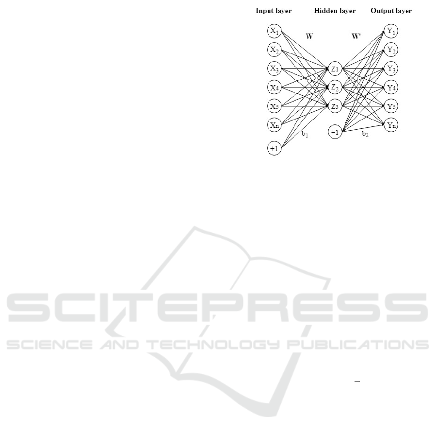
3.1 Autoencoders
The autoencoder is a neural network that aims to le-
arn a more suitable representation of the data, usually
by reducing its dimension (Goodfellow et al., 2016).
It is trained in an unsupervised manner to reconstruct
the input by minimizing the error between the input
and the output. We can split the network in two parts:
the encoder function, where the encoding of the input
is done, and the decoder function, where it tries to re-
construct the input from the code obtained by the en-
coder. The purpose of the reconstruction is to obtain a
useful compressed representation (the "code") which
will be usable as input of a classifier. As we can see
in Figure 1, the encoder function f maps an input
X to a hidden representation Z. Then, the decoder
function g maps the hidden representation Z to an in-
put reconstruction Y . Usually f and g are nonlinear
functions (sigmoid or hyperbolic tangent). The enco-
der and decoder output are described in the Equation
1 and Equation 2 respectively, where W,W
0
, b
1
, b
2
are
the learnable parameters.
Z = f (W X + b
1
) (1)
Y = g(W
0
Z + b
2
) (2)
The minimization of the reconstruction error is
done during the training phase. For real-valued output
Figure 1: Diagram of a basic autoencoder.
we usually use the square-error loss function (Eq. 3)
and for binary output the cross-entropy loss function
is normally used (Eq. 4).
L
SE
(θ;X) =
n
∑
i=1
|| x
i
− y
i
||
2
(3)
L
CE
(θ;X) = −
n
∑
i=1
[x
i
log(y
i
)+(1−x
i
)log(1−y
i
))]
(4)
where θ = (W,W
0
, b
1
, b
2
) and n is the total number of
input data.
We usually add to the loss function a regulariza-
tion term, also called weight-decay, to penalize large
weights and avoid the overfitting as:
L(θ;X) = L(θ;X) +
λ
2
|| W ||
2
(5)
where L represents the square-error or cross-entropy
loss function and λ is the regularization parameter.
3.2 Support Vector Machine
Support Vector Machine (SVM) is a supervised lear-
ning method proposed by (Cortes and Vapnik, 1995)
for solving classification or regression problems. The
simplest case is when data belong to only two classes.
The SVM will be trained to find a hyperplane that best
separates these classes, which is mathematically des-
cribed as:
f (x) = w
T
x + b (6)
and the decision function as:
y = sign(w
T
x + b) (7)
where x ∈ χ is the input data, y ∈
{
−1, 1
}
is the out-
put class and w, b the learnable parameters. The dis-
tance between this hyperplane and the nearest sample
Deep Learning-based Method for Classifying and Localizing Potato Blemishes
109

is called margin. The larger the margin, the better
ability to generalize has the model and that is why the
SVM looks for the optimal hyperplane that maximi-
zes the margin. To determine the optimal hyperplane,
we look for the minimum distance between the hyper-
plane and the closest example of each class (positive
and negative class). Finally, the optimal hyperplane
can be found if we solve the quadratic problem of li-
near constraints that follows:
min
w,ξ
1
2
k
w
k
2
+C
n
∑
i=1
ξ
i
!
, C ≥ 0 (8)
subject to
y
i

w
T
x
i
+ b

≥ 1 − ξ
i
, ∀i = 1, ..., n (9)
ξ
i
≥ 0, ∀i = 1, ..., n (10)
where n is the size of input data, C is the penalization
parameter that we can modify in order to accept more
or less inaccurate classification and ξ
i
a slack variable.
To solve the minimization problem of Eq. 8, we use
the dual formulation:
max
α
n
∑
i=1
α
i
−
1
2
n
∑
i, j=1
α
i
α
j
y
i
y
j
x
T
i
x
j
!
(11)
subject to
n
∑
i=1
α
i
y
i
= 0, (12)
0 ≤ α
i
≤ C, ∀i = 1, ..., n (13)
And the decision function:
y = sign
∑
i∈SV
α
i
y
i
x
T
x
i
+ b
!
(14)
where SV are the support vectors, i.e, samples for
which 0 < α
i
< C.
To adapt the SVM to non-linear problems we re-
place the function φ(x, x
i
) = x
T
x
i
by a kernel function
defined as:
K (x, x
i
) =
h
φ(x), φ(x
i
)
i
(15)
where φ(x) is the mapping function that project the
input data χ to a new feature space ν where a linear
solution exists.
3.3 Convolutional Neural Networks
A Convolutional Neural Network (CNN) is a type of
neural network consisting of a sequence of layers that
convolve the inputs to obtain useful information (Le-
Cun et al., 1990). Convolutional, pooling and fully-
connected layers are the main layers that we can find
in these networks. The convolutional layer convol-
ves the input image with the kernel filter in a sliding-
window manner. The filters are the learnable parame-
ters of the network. By this operation, the features of
the input image are extracted and the output is nor-
mally called Activation map or Feature map. After
the convolution, an activation function is applied to
introduce non-linearity in the CNN. Rectified Linear
Unit (ReLU) is generally applied, which is defined as:
f (x) = max(0, x) (16)
The output obtained by a convolution operation is cal-
culated as follows:
z
l
j
= f (
∑
i∈M
j
x
l−1
i
×W
l
i j
+ b
l
j
) (17)
where z
l
j
is the output of neuron j in convolutional
layer l, f is the activation function, M
j
is the set of
input features, x
l−1
i
is the input feature of layer l − 1,
W
l
i j
is the ith weight of neuron j in layer l, and b
l
j
is the bias of jth neuron in lth layer. The pooling
operation is then applied in order to reduce dimensi-
onality and acquire spatial invariant features (Scherer
et al., 2010). Max pooling and average pooling are
examples of commonly use pooling operators. The
first one applies a max-filter to sub-regions of the pre-
vious layer representation in order to keep the maxi-
mum value of each sub-region. The second one, ap-
plies an average-filter resulting in an average value of
each sub-region. At the end, a fully-connected (FC)
layer can be applied for high-level reasoning. Each
neuron of this FC layer is connected to all neurons of
the previous layer. For classification, the output of the
last FC layer pass through an output function, like a
softmax function.
3.4 Overall Scheme of Proposed
Method
Figure 2 presents the overview of the proposed met-
hod. It is composed by three main phases. Firstly, a
CNN was trained to classify face potato images and to
select faces where defects must be localized, i.e. da-
maged and greening faces. Secondly, a combination
of autoencoder and SVMs was applied on the selected
images to localize defects in a patch-wise manner. Fi-
nally, in the third phase, we used the localization re-
sults of the previous phase to train two SVMs to clas-
sify damaged and greening potatoes by defect gravity.
A detailed explanation of each phase is presented:
(a) Training for classification: we fine-tuned a
pre-trained CNN with our training dataset
to classify the images in 6 distinct classes.
ICPRAM 2019 - 8th International Conference on Pattern Recognition Applications and Methods
110

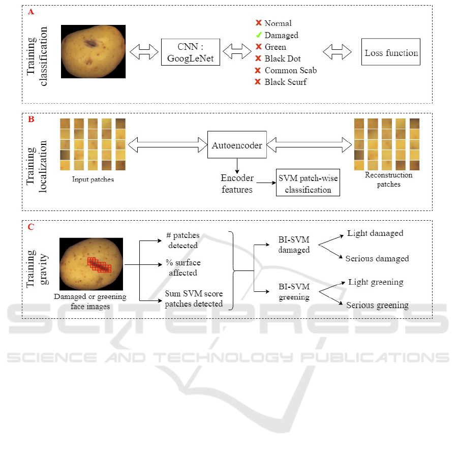
Figure 2: Scheme of the proposed method.
Three powerful pre-trained deep neural net-
works were tested to keep the one who best
suits our problem (AlexNet (Krizhevsky et al.,
2012), VGG-16 (Simonyan and Zisserman,
2014) and GoogLeNet (Szegedy et al., 2015)).
All of them were trained on ImageNet (Deng
et al., 2009), a dataset of more than 1 mil-
lion images of 1000 classes. In order to fine-
tune the pre-trained network, we replaced its
last fully-connected layer of 1000 output clas-
ses, by a new one that classifies the images in
6 classes. We obtained the best results with
GoogLeNet (more details about the network
selection are in Section 4.1). The CNN was
used to classify potato faces and also selects
the images that will move on to the next step
for further analyses. Because of the whole
image analysis, this method allows us to take
into account the context information, which
was not possible to achieve with patch-wise
processing. For example, the extensive di-
versity in potatoes makes difficult to analyze
the appearance of defects only based on small
regions. Furthermore, the CNN reduced the
number of images that would be processed in
the second stage by selecting only the images
where a defect must be localized, i.e. dama-
ged or greening potatoes. Nevertheless, we
compared the results obtained with and wit-
hout the CNN classification to better under-
stand the usefulness of this phase.
(b) Training for localization: to classify green-
ing and damaged potatoes by gravity we need
to identify the size of the surface affected
by the defect. We trained an autoencoder
with 16×16 patches extracted from images,
excluding background. The encoder featu-
res were then used to train two binary Sup-
port Vector Machine (SVM) classifiers which
were used to classify patches into damaged or
non-damaged and greening or non-greening
respectively. The classification was done in
a sliding window manner to obtain an accu-
rate segmentation of the defect. The impor-
tant computation resource consumed by the
sliding-window approach is reduced by the
preselection accomplished by the CNN in the
previous stage.
(c) Training for gravity classification: after the
Deep Learning-based Method for Classifying and Localizing Potato Blemishes
111

previous stages (a) and (b), we used the in-
formation of the patches identified as defects
(damaged or greening) for training the last bi-
nary SVM classifiers which divide the dama-
ged and greening images by gravity: light or
serious. The input used for the SVMs was: (1)
the number of patches detected, (2) the per-
centage of the surfaced affected and (3) the
sum of SVM output score of detected patches.
3.5 Training, Validation and Test
Dataset
A large dataset was created to train, validate and test
the proposed method. Different cameras were used in
order to take 4 RGB images of different potato faces.
The images were taken with a black background. Po-
tatoes of different varieties (Agata, Libertie, Caesar,
Monalisa, Gourmandine, Annabelle, Charlotte, Ma-
rilyn), shape and size were used to create a dataset
of 9688 images which come from 2422 tubers. The
images were manually classified with the help of two
experts. Two different classifications were performed:
firstly the potato was classified with its 4 faces toget-
her in 8 distinct classes: healthy, light damaged, seri-
ous damaged, light greening, serious greening, black
dot, common scab and black scurf. Secondly, all faces
were classified separately in order to train the CNN by
using individual face images. In the face-wise classi-
fication, only 6 classes were taken into account be-
cause light and serious defects group together. As we
show in Table 1, the final distribution for face-image
classification was: 5325 healthy, 984 damaged, 1263
greening, 597 black dot, 1276 common scab and 243
of black scurf. An example of these images is illustra-
ted in Figure 3. On the other hand, Table 2 show the
distribution of potato images classification: 831 he-
althy, 341 light damaged, 159 serious damaged, 161
light greening, 349 serious greening, 151 black dot,
359 common scab and 71 of black scurf. Only green
and damaged potatoes were divided by gravity be-
cause of sample availability. 30% of dataset was rand-
omly selected for testing the proposed method. The
remaining was used for training and validate the mo-
dels. The 4 face images of the same potato were all in
the same set. To fine-tune the pre-trained CNN, ima-
ges were resized to pre-defined input size of each net-
work (227×227 for AlexNet and 224×224 for VGG-
16 and GoogLeNet). Data augmentation techniques
as flipping and rotation were randomly applied in or-
der to increase the amount of training examples and
its variability. To train the autoencoder, we extrac-
ted 29657 random 16x16 patches from 168 images.
All patches that had background pixels were not ta-
Table 1: Face-wise image classification dataset.
Class Number of images
Healthy 5325
Damaged 984
Greening 1263
Black dot 597
Common scab 1276
Black scurf 243
Total 9688
Table 2: Potato-wise image classification dataset.
Class Number of images
Healthy 831
Light damaged 341
Serious damaged 159
Light greening 161
Serious greening 349
Black dot 151
Common scab 359
Black scurf 71
Total 2422
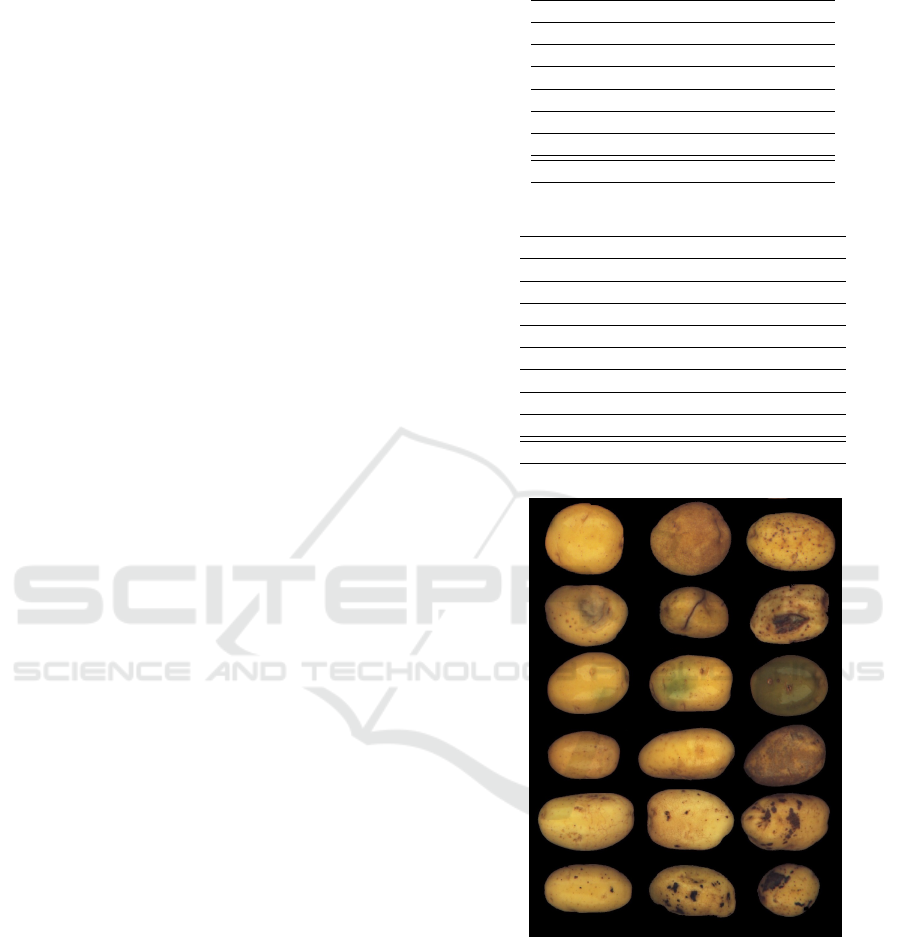
Figure 3: Example of the six distinct classes with variable
gravity. By rows, from top to bottom: healthy, damaged,
greening, black dot, common scab and black scurf.
ken into account. This decision was made after some
experiments in which border patches were classified
as damaged. To classify the patches between dama-
ged or non-damaged and green or non-green, a labe-
led dataset was created. From 115 damaged face ima-
ges, 3962 damaged patches and 14249 non-damaged
patches were extracted. Then, for 100 greening face
images, 1271 green patches and 7722 non-green pat-
ches were labeled.
ICPRAM 2019 - 8th International Conference on Pattern Recognition Applications and Methods
112

3.6 Evaluation Metrics
The evaluation metrics used in this work were se-
lected in order to take into account the imbalanced
nature of the dataset (Bekkar et al., 2013). They are
described as follows:
• Confusion matrix: compare the predicted clas-
ses with the real classes. Each column represents
the ground-truth class and each row represents the
classifier prediction.
• Precision
k
:
P
k
=
T P
k
T P
k
+ FP
k
(18)
• Recall
k
:
R
k
=
T P
k
T P
k
+ FN
k
(19)
• F1-score
k
:
F1 − score
k
= 2 ∗
P
k
∗ R
k
P
k
+ R
k
(20)
where T P
k
is true positives of class k, FP
k
is false
positives of class k and FN
k
is false negatives of class
k.
In the localization phase, we used the False Alarm
Rate (FAR) and False Negative Rate (FNR) calculated
as following:
FAR =
Number o f f alse positives
Total number o f negatives
(21)
FNR =
Number o f f alse negatives
Total number o f positives
(22)
4 RESULTS AND DISCUSSION
We evaluated the performance of the proposed met-
hod on the three main stages. We show that our propo-
sed method classifies and localizes blemishes with sa-
tisfactory results. Implementation was made in Mat-
lab R2017b. All experiments were done using a GPU
NVIDIA GEFORCE GTX 1050 Ti (4 GB memory).
4.1 Face Image Classification
We fine-tuned and compared results of three powerful
pre-trained CNN: AlexNet (Krizhevsky et al., 2012),
VGG-16 (Simonyan and Zisserman, 2014) and Goo-
gLeNet (Szegedy et al., 2015). Stochastic gradient
descent with momentum set in 0.9 was used to fine-
tuned networks. The learning rate of the new fully-
connected layer was 20 times the global learning rate
set to 0.0001. The mini-batch size was set to 10 due
to memory limitation of our GPU and the maximum
number of epochs was limited to 100. The cross-
validation technique with 5-folds was used. We di-
vided the training set in five equal parts and we fine-
tuned the network using four parts, leaving the remai-
ning part to validate the results. The process was re-
peated five times and the mean and standard devia-
tion F1-score per class is shown in Table 3. It can
be observed that GoogLeNet results are slightly bet-
ter for all classes resulting in an average F1-score of
0.94 against to 0.92 and 0.88 for AlexNet and VGG-
16 respectively. Table 4 shows the confusion matrix
obtained using GoogLeNet architecture. It compares
the predicted classes with the ground truth data. The
biggest confusion occurred between black dot and he-
althy face images. This usually happens when the di-
sease is not evident or it is near the border. Based
on these results, we used the fine-tuned GoogLeNet
as a classification filter, in order to classify each face
image and pass through the localization phase only
the damaged and greening.
Table 3: F1-score results in face image classification. Clas-
ses are: H=Healthy, D=Damaged, G=Greening, BD=Black
Dot, CS=Common Scab and BS=Black Scurf.
Classes AlexNet VGG-16 GoogLeNet
H 0.95 ± 0.02 0.94 ± 0.07 0.97 ± 0.01
D 0.92 ± 0.03 0.88 ± 0.03 0.94 ± 0.02
G 0.96 ± 0.04 0.95 ± 0.01 0.98 ± 0.02
BD 0.82 ± 0.04 0.76 ± 0.03 0.85 ± 0.06
CS 0.93 ± 0.03 0.90 ± 0.01 0.96 ± 0.02
BS 0.93 ± 0.04 0.86 ± 0.04 0.95 ± 0.04
Table 4: Confusion matrix using GoogLeNet architec-
ture in face image classification. Classes are: H=Healthy,
D=Damaged, G=Greening, BD=Black Dot, CS=Common
Scab and BS=Black Scurf.
Ground-Truth(%)
H D G BD CS BS
Pred.(%)
H 98.1 6.3 2.8 20.5 3.7 1.1
D 0.6 92.4 0.0 0.2 0.3 0.6
G 0.2 0.1 96.9 0.5 0.1 0.0
BD 0.6 0.0 0.2 78.4 0.2 0.0
CS 0.4 1.0 0.1 0.5 94.5 1.1
BS 0.1 0.1 0.0 0.0 1.1 97.1
4.2 Defect Localization
The autoencoder with 50 neurons in the hidden layer
was trained using scaled conjugate gradient descent,
means squared error loss function and weight decay
λ = 3 × 10
−6
. The sigmoid function was used as acti-
vation function. As depict in Figure 4, the patches
reconstruction made by the autoencoder was success-
fully achieved.
Deep Learning-based Method for Classifying and Localizing Potato Blemishes
113

Figure 4: Comparison of test patches and their recon-
struction made by the autoencoder.
To detect damaged and green patches we trained
two binary SVM classifiers, one for each classifica-
tion task. Cross-validation with 5-fold was also ap-
plied. In addition, grid search was used in order to
tune the hyperparameters, i.e. choose the combina-
tion of the Gaussian kernel parameter σ and C that
maximized the performance in the validation set. We
compared the results between binary SVM (BI-SVM)
and one class SVM (OC-SVM). The main idea to ap-
ply OC-SVM was the ease of obtaining only normal
patches (without defects). Table 5 shows the results
on damaged dataset and Table 6 shows the results on
greening dataset. As expected, we noticed a great
improvement in the results when using BI-SVM. We
obtained a similar FAR with a considerable decrease
of FNR in both, damaged and greening classification.
Table 5: Patches classification results. Damaged versus
non-damaged patches.
FAR(%) FNR(%)
OC-SVM 4.23 27.66
BI-SVM 4.19 14.46
Table 6: Patches classification results. Greening versus non-
greening patches.
FAR(%) FNR(%)
OC-SVM 4.91 39.11
BI-SVM 5.53 28.11
4.3 Classification by Gravity
In this phase we classified damaged and greening
images by gravity. Only healthy, damaged and green-
ing potatoes were used to train and validate the mo-
dels. The 16×16 overlapping patches were extrac-
ted with a stride of 8 and they were used as input for
the autoencoder as explained in Section 4.1. Figure
5 shows an example of the localization made by the
autoencoder+SVM. The localization output was then
used as input of the SVM classifier. Until this phase a
face-wise classification was done, but to classify de-
fect gravity of the whole potato we needed to take into
account the four faces of that potato. Thus, to charac-
terize the whole potato image we only retained the lo-
calization results of the face where the biggest defect
was detected. For example, if two faces of the same
potato were classified as damaged, we only use the
localization results from the face where we have loca-
lized the biggest defect. Finally, potato images were
classified in Light Damaged (LD) or Serious Dama-
ged (SD) and Light Greening (LG) or Serious Green-
ing (SG). Cross-validation and grid search were app-
lied. The input features used were:
(1) Number of patches detected by autoenco-
der+SVM.
(2) Percentage of the surface detected as dama-
ged or greening by autoencoder+SVM. (
ND
NT
,
where ND is the number of detected patches
and NT is the total number of patches extrac-
ted from the face image).
(3) The sum of the SVM output score of all de-
tected patches.
Figure 5: Example of damaged (left) and greening (right)
localization output of autoencoder+SVM models. Blue pa-
tch depicts an isolate patch, where no adjacent patch is de-
tected. In this case, the blue patch is discarded in order to
minimize false alarms and avoid the detection of small de-
fects.
Table 7 and Table 8 show the results of damaged
and greening gravity classification respectively. We
compare the results obtained with and without using
the CNN as a first classification step. When the CNN
is not used, an image is classified as healthy if less
than two defect patches are detected. Better results
were achieved when using the CNN, decreasing the
number of healthy potatoes classified as damaged or
greening. Another advantage of using the CNN as
first classification step is the reduction of computing
time. The CNN prediction is two times faster than
the autoencoder+SVM patch-wise defect localization
method. That is why analyzing only damaged and
greening face images in the localization stage greatly
reduces the processing time. We conclude according
to the results that features extracted from the localiza-
tion of Section 4.2 are useful for classifying by gravity
ICPRAM 2019 - 8th International Conference on Pattern Recognition Applications and Methods
114

the damaged and greening potato images. The confu-
sion matrices of each classification task, without and
with the use of the CNN, are shown in Table 9 and
Table 10. As shown in Table 9, only 0.91% (1 potato)
of serious damaged potato was predicted as healthy,
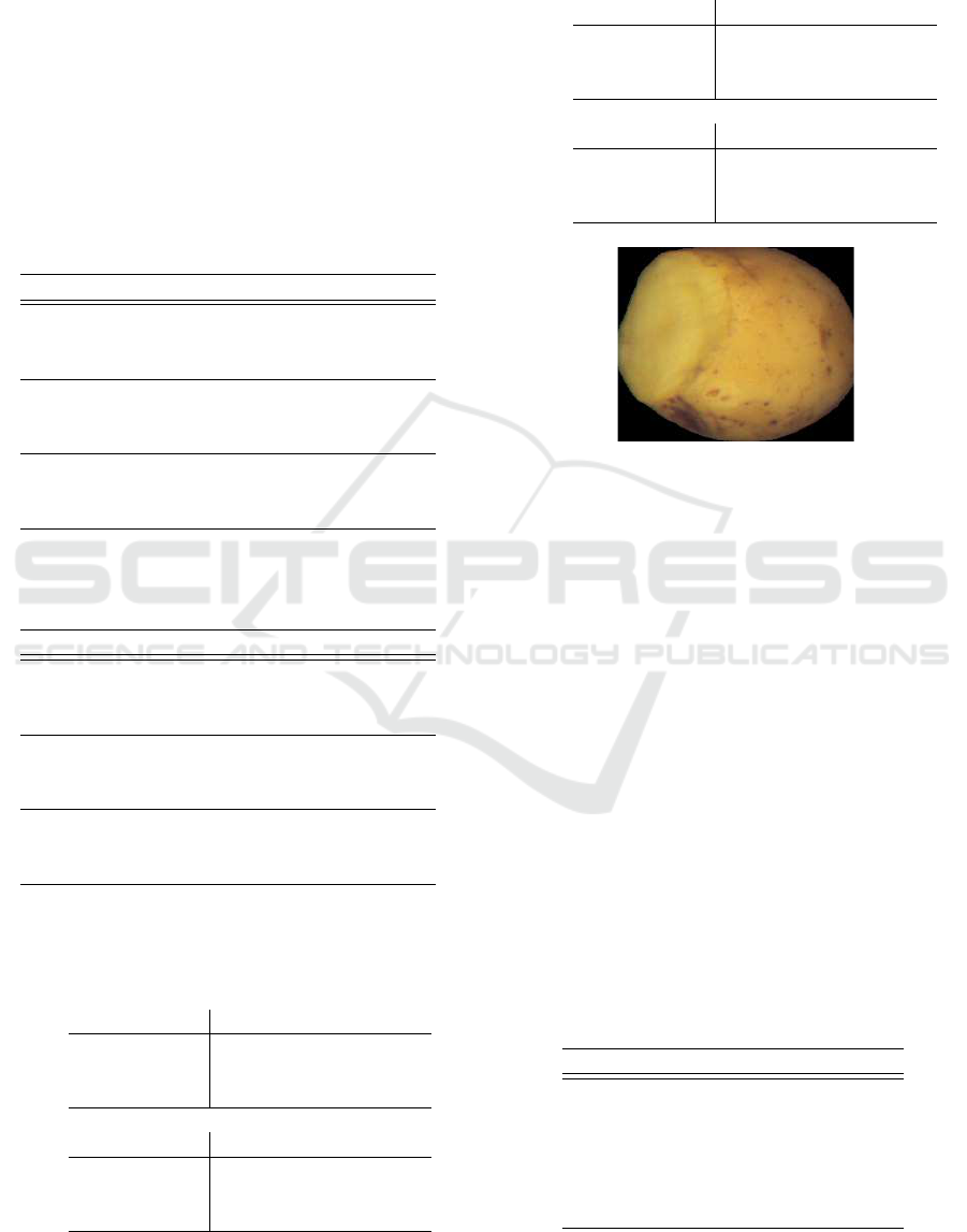
which is the most critical mistake. That occurred with
a cutted potato, where the damaged portion was not
dark but light yellow (see Figure 6). A great impro-
vement on the false alarms is achieved with the use of
the CNN from 7.55% to 0.69% and 15.78% to 0% for
damaged and greening potato images respectively.
Table 7: Cross-validation results for potato images divided
between Healthy (H), Light Damaged (LD) and Serious Da-
maged (SD).
without CNN with CNN
Precision
H 0.96 0.97
LD 0.80 0.94
SD 0.95 0.94
Recall
H 0.92 0.99
LD 0.88 0.91
SD 0.93 0.90
F1-score
H 0.94 0.98
LD 0.84 0.92
SD 0.94 0.92
Table 8: Cross-validation results for potato images divi-
ded between Healthy (H), Light Greening (LG) and Serious
Greening (SG).
without CNN with CNN
Precision
H 0.99 0.99
LG 0.37 0.86
SG 0.88 0.96
Recall
H 0.84 1
LG 0.62 0.85
SG 0.98 0.95
F1-score
H 0.91 0.99
LG 0.47 0.85
SG 0.93 0.95
Table 9: Confusion matrix for potato images divided bet-
ween Healthy (H), Light Damaged (LD) and Serious Da-
maged (SD).
Ground-Truth(%)
without CNN H LD SD
Pred.(%)
H 92.28 10.50 0
LD 7.55 87.82 7.27
GD 0.17 1.68 92.73
with CNN H LD SD
Pred.(%)
H 99.31 6.72 0.91
LD 0.69 90.76 9.09
GD 0 2.52 90.00
Table 10: Confusion matrix for potato images divided bet-
ween Healthy (H), Light Greening (LG) and Serious Green-
ing (SG).
Ground-Truth(%)
without CNN H LG SG
Pred.(%)
H 83.70 4.30 0
LG 15.78 62.37 2.28
GG 0.51 33.33 97.72
with CNN H LG SG
Pred.(%)
H 100 3.23 0
LG 0 84.95 4.94
GG 0 11.83 95.06
Figure 6: Example of miss-detection of a serious damaged
potato.
4.4 Multi-class Multi-label
Classification
For the final results, a multi-class multi-label test da-
taset of 722 tubers was available. We took into ac-
count the four output labels obtained in the previous
stages, one per face image, to characterize the whole
potato. The final results with and without gravity
classification are shown in Table 11 and Table 12 re-
spectively. We observe that despite the similarity bet-
ween some classes and the high variability within the
same class, the whole system performs well. The he-
althy class achieved the best performance with a cor-
rect prediction of 98%, showing that the number of
false alarms was small. Black dot had the smallest
detection results (82%) due to the confusion with he-
althy images (as seen in Section 4.1).
Table 11: Test multi-class multi-label dataset results.
H=Healthy, D=Damaged, G=Greening, BD=Black Dot,
CS=Common Scab and BS=Black Scurf.
Precision Recall F1-score
H 0.98 0.98 0.98
D 0.93 0.97 0.95
G 1 0.99 0.99
BD 0.92 0.82 0.87
CS 0.95 0.87 0.91
BS 0.88 0.95 0.91
Deep Learning-based Method for Classifying and Localizing Potato Blemishes
115

Table 12: Test multi-class multi-label dataset results.
H=Healthy, LD=Light Damaged, SD= Serious Damaged,
LG=Light Greening, SG=Serious Greening, BD=Black
Dot, CS=Common Scab and BS=Black Scurf.
Precision Recall F1-score
H 0.98 0.98 0.98
LD 0.90 0.94 0.92
SD 0.86 0.88 0.87
LG 0.88 0.91 0.89
SG 0.98 0.95 0.96
BD 0.92 0.82 0.87
CS 0.95 0.87 0.91
BS 0.88 0.95 0.91
5 CONCLUSION AND FUTURE
WORK
In this work we present a new three stages deep
learning-based method which is able to classify and
localize blemishes in potatoes, resulting in a global
evaluation of the tuber. A large database has been
created including healthy and 5 distinct blemishes,
i.e., damaged, greening, black dot, common scab and
black scurf. A Convolutional Neural Network has
been trained with this database. This network is used
as the first stage of our method for classifying the face
potato images and selecting those images where de-
fects must be localized, i.e. damaged and greening.
A second stage has been applied on the selected ima-
ges, where a combination of autoencoder and SVMs
is used to detect damaged and greening defects in a
patch-wise manner. Finally, in the third stage, locali-
zation results have been used to train two SVMs for
grading damaged and greening potatoes according to
the severity of the blemish.
Results showed that we could accurately classify
face potato images within 6 classes with an average
precision of 95% and average recall of 93%. A
patch-wise analysis was done to localize damaged and
greening parts of the potato achieving a false positive
rate of 4.19% and 5.53% respectively. The final glo-
bal evaluation of the tuber reached an average preci-
sion of 92% and average recall of 91% in a test set.
The speed and efficiency of our method allow us to
use it in a real industrial setting. In addition it does not
require a pixel-level labeling, which is laborious and
time-consuming. Despite other works have been pro-
posed to classify potatoes, unavailability of public im-
plementations make it difficult to have a comparative
study. Furthermore, previous works have used limi-
ted databases in terms of number of examples and/or
number of defects to classify, which makes it difficult
to make a fair comparison to other algorithms.
Future studies will investigate the improvement
of the blemishes segmentation by using a non-
supervised method applicable to the whole image.
The ability to recognize multiple blemishes will be
studied. Also, an update of the dataset will be made
to increase the effectiveness of the proposed method.
Finally, the use of 3D tuber images will be explored,
where the whole surface will be analyzed at once, wit-
hout using multiple face images per potato.
REFERENCES
Badrinarayanan, V., Kendall, A., and Cipolla, R. (2015).
Segnet: A deep convolutional encoder-decoder ar-
chitecture for image segmentation. arXiv preprint
arXiv:1511.00561.
Barnes, M., Duckett, T., Cielniak, G., Stroud, G., and Har-
per, G. (2010). Visual detection of blemishes in pota-
toes using minimalist boosted classifiers. Journal of
Food Engineering, 98(3):339–346.
Bekkar, M., Djemaa, H. K., and Alitouche, T. A. (2013).
Evaluation measures for models assessment over im-
balanced datasets. Iournal Of Information Engineer-
ing and Applications, 3(10).
Blasco, J., Aleixos, N., and Molto, E. (2007). Computer
vision detection of peel defects in citrus by means of
a region oriented segmentation algorithm. Journal of
Food Engineering, 81(3):535–543.
Bolle, R. M., Connell, J. H., Haas, N., Mohan, R., and Tau-
bin, G. (1996). Veggievision: A produce recognition
system. In Applications of Computer Vision, 1996.
WACV’96., Proceedings 3rd IEEE Workshop on, pa-
ges 244–251. IEEE.
Brahimi, M., Boukhalfa, K., and Moussaoui, A. (2017).
Deep learning for tomato diseases: classification and
symptoms visualization. Applied Artificial Intelli-
gence, 31(4):299–315.
Cortes, C. and Vapnik, V. (1995). Support-vector networks.
Machine learning, 20(3):273–297.
Dacal-Nieto, A., Vázquez-Fernández, E., Formella, A.,
Martin, F., Torres-Guijarro, S., and González-Jorge,
H. (2009). A genetic algorithm approach for fea-
ture selection in potatoes classification by computer
vision. In Industrial Electronics, 2009. IECON’09.
35th Annual Conference of IEEE, pages 1955–1960.
IEEE.
Deng, J., Dong, W., Socher, R., Li, L.-J., Li, K., and Fei-
Fei, L. (2009). ImageNet: A Large-Scale Hierarchical
Image Database. In CVPR09.
ElMasry, G., Cubero, S., Moltó, E., and Blasco, J. (2012).
In-line sorting of irregular potatoes by using automa-
ted computer-based machine vision system. Journal
of Food Engineering, 112(1-2):60–68.
Goodfellow, I., Bengio, Y., Courville, A., and Bengio, Y.
(2016). Deep learning, volume 1. MIT press Cam-
bridge.
ICPRAM 2019 - 8th International Conference on Pattern Recognition Applications and Methods
116

Hinton, G., Deng, L., Yu, D., Dahl, G. E., Mohamed, A.-
r., Jaitly, N., Senior, A., Vanhoucke, V., Nguyen, P.,
Sainath, T. N., et al. (2012). Deep neural networks for
acoustic modeling in speech recognition: The shared
views of four research groups. IEEE Signal processing
magazine, 29(6):82–97.
Hu, M.-h., Dong, Q.-l., Liu, B.-l., and Malakar, P. K.
(2014). The potential of double k-means clustering
for banana image segmentation. Journal of Food Pro-
cess Engineering, 37(1):10–18.
IPC (2018). International potato center. https://cipotato.org.
Accessed: 04 Septembre 2018.
Jhuria, M., Kumar, A., and Borse, R. (2013). Image proces-
sing for smart farming: Detection of disease and fruit
grading. In Image Information Processing (ICIIP),
2013 IEEE Second International Conference on, pa-
ges 521–526. IEEE.
Krizhevsky, A., Sutskever, I., and Hinton, G. E. (2012).
Imagenet classification with deep convolutional neu-
ral networks. In Advances in neural information pro-
cessing systems, pages 1097–1105.
LeCun, Y., Boser, B. E., Denker, J. S., Henderson, D.,
Howard, R. E., Hubbard, W. E., and Jackel, L. D.
(1990). Handwritten digit recognition with a back-
propagation network. In Advances in neural informa-
tion processing systems, pages 396–404.
Miller, B. K. and Delwiche, M. J. (1989). A color vision
system for peach grading. Transactions of the ASAE,
32(4):1484–1490.
Ming, W., Du, J., Shen, D., Zhang, Z., Li, X., Ma, J. R.,
Wang, F., and Ma, J. (2018). Visual detection of
sprouting in potatoes using ensemble-based classifier.
Journal of Food Process Engineering, 41(3):e12667.
Mohanty, S. P., Hughes, D. P., and Salathé, M. (2016).
Using deep learning for image-based plant disease de-
tection. Frontiers in plant science, 7:1419.
Noordam, J. C., Otten, G. W., Timmermans, T. J., and van
Zwol, B. H. (2000). High-speed potato grading and
quality inspection based on a color vision system. In
Machine Vision Applications in Industrial Inspection
VIII, volume 3966, pages 206–218. International So-
ciety for Optics and Photonics.
Oppenheim, D. and Shani, G. (2017). Potato disease classi-
fication using convolution neural networks. Advances
in Animal Biosciences, 8(2):244–249.
Picon, A., Alvarez-Gila, A., Seitz, M., Ortiz-Barredo, A.,
Echazarra, J., and Johannes, A. (2018). Deep con-
volutional neural networks for mobile capture device-
based crop disease classification in the wild. Compu-
ters and Electronics in Agriculture.
Redmon, J., Divvala, S., Girshick, R., and Farhadi, A.
(2016). You only look once: Unified, real-time object
detection. In Proceedings of the IEEE conference on
computer vision and pattern recognition, pages 779–
788.
Scherer, D., Müller, A., and Behnke, S. (2010). Evaluation
of pooling operations in convolutional architectures
for object recognition. In Artificial Neural Networks–
ICANN 2010, pages 92–101. Springer.
Simonyan, K. and Zisserman, A. (2014). Very deep con-
volutional networks for large-scale image recognition.
arXiv preprint arXiv:1409.1556.
Szegedy, C., Liu, W., Jia, Y., Sermanet, P., Reed, S., Angue-
lov, D., Erhan, D., Vanhoucke, V., and Rabinovich, A.
(2015). Going deeper with convolutions. In Procee-
dings of the IEEE conference on computer vision and
pattern recognition, pages 1–9.
Tao, Y., Heinemann, P., Varghese, Z., Morrow, C., and Som-
mer Iii, H. (1995). Machine vision for color inspection
of potatoes and apples. Transactions of the ASAE,
38(5):1555–1561.
Vízhányó, T. and Felföldi, J. (2000). Enhancing colour dif-
ferences in images of diseased mushrooms. Compu-
ters and Electronics in Agriculture, 26(2):187–198.
Xing, J., Bravo, C., Jancsók, P. T., Ramon, H., and De Baer-
demaeker, J. (2005). Detecting bruises on ‘golden de-
licious’ apples using hyperspectral imaging with mul-
tiple wavebands. Biosystems Engineering, 90(1):27–
36.
Xiong, J., Tang, L., He, Z., He, J., Liu, Z., Lin, R., and Xi-
ang, J. (2017). Classification of potato external quality
based on svm and pca. International Journal of Per-
formability Engineering, 17(4):469.
Zaborowicz, M., Boniecki, P., Koszela, K., Przybylak, A.,
and Przybył, J. (2017). Application of neural image
analysis in evaluating the quality of greenhouse toma-
toes. Scientia Horticulturae, 218:222–229.
Zhou, L., Chalana, V., and Kim, Y. (1998). Pc-based ma-
chine vision system for real-time computer-aided po-
tato inspection. International journal of imaging sys-
tems and technology, 9(6):423–433.
Deep Learning-based Method for Classifying and Localizing Potato Blemishes
117