Context-based User Activity Prediction for Mobility Planning

Karl-Heinz Krempels

1,2

, Fabian Ohler

1,2

, Thomas Osterland

and Christoph Terwelp

1,2

Informatik 5 Information Systems, RWTH Aachen University, Aachen, Germany

Fraunhofer-Institut f

ur Angewandte Informationstechnik FIT, Sankt Augustin, Germany

Keywords:

Mobility Planning, Activity Prediction, Next Location Prediction.

Abstract:

By analyzing the individual travel characteristics of persons, it occurs that most trips are not journeys to other

cities or countries but short trips, as the daily trip to work or the weekly meeting at the gym. For those trips,

people know the basic conditions, as e.g., the bus driving schedule or the journey duration and it represents

more effort to plan the trip beforehand, than just remember the data. But what if there is a problem, like a

stalled train or a car crash on the route. Unpredictable ocurrences might be noticed too late and affect the

parameters of the trip. A travelling assistant that is able to anticipate regular trips and that warns in case of

problems, without requesting dedicated user input might be a solution.

In this paper we consider the problem of creating an assistant based on the context information captured from

a smartphone. We discuss approaches based on histogram evaluation, a Bayesian network and a multilayer

perceptron that allow the prediction of locations and activities given a time and a date. These approaches are

benchmarked and compared to each other to ﬁnd the solution that provides the best results in prediction quality

and training speed.

1 INTRODUCTION

Providing assistance in the planning of trips is an ela-

borately researched topic and subject of a large num-

ber of publications. Therein the focus often lies on

long journeys, like trips to different countries or to

another city. Often the assistance only extends to pro-

viding input form proposals, as proposing the name

of a city that a person often visited in the past.

Instead we focus on regular trips on a daily base,

as the daily trip to work or the weekly meeting at the

gym. These are trips a person travels repeatedly and

the basic conditions of the route, as e.g., the bus line

or the departure time, are learned and memorized.

If a person uses the bus for the daily ride to work

she knows that the bus departs at 8 a.m. and that she

has to leave the house at 7.55 a.m. A person following

this routine every day will not check the route for pos-

sible problems, as e.g., a bus cancellation, since most

of the time it is unnecessary effort.

Our interest is focused of answering the following

question: Is it possible to observe daily routes and au-

tomatically provide information about potential pro-

blems without additional user interaction?

We build an Android App that runs on mobile de-

vices and captures context information (timestamp,

location, calendar information, etc.) every 15 minu-

tes. We notice that providing automatic travel assis-

tance is about knowing the location and activity of a

person for every point in time – particularly for times

lying in the future. Thus the challenge is to identify

an approach that predicts the context of a person gi-

ven a date in the future, while trained with data from

the past. Besides, additional constraints regarding the

learning speed and the accuracy need to be conside-

red, since a user can not train the system half a year

before actually beneﬁt from it. Also the adaptability

of the system is important to react on changes in the

daily routine as moving to another city or quitting the

job.

To enable more personalized travel assistance we

additionally provide a mechanism to extend the loca-

tion information by recognizing and labeling them as

home or work location.

After the introduction in Section 1, we provide an

overview of existing similar approaches in Section 2.

In Section 3 we introduce three different approaches

that are able to predict the activity and location of

a person based on training data. We introduce a

rating-based mapping function that allows the identi-

ﬁcation of the home and work location and provide

benchmark results of the considered approaches in

Section 5. A conclusion of the results and a short out-

look is given in Section 6.

568

Krempels, K., Ohler, F., Osterland, T. and Terwelp, C.

Context-based User Activity Prediction for Mobility Planning.

DOI: 10.5220/0007351105680575

In Proceedings of the 11th International Conference on Agents and Artiﬁcial Intelligence (ICAART 2019), pages 568-575

ISBN: 978-989-758-350-6

2 RELATED WORK

The concept of personal travel assistants (PTA) is

introduced in (Foundation for Intelligent Physical

Agents, 2001). They describe an agent that learns and

follows the user’s instructions and acts like a real phy-

sical personal assistant. In this way the agent supports

the user in trip planning and execution.

Thereby the PTA aims at rather more comprehen-

sive journeys than daily travel and the training is ba-

sed on formerly done trips instead of continuously

captured device context information.

Automatic travel assistance systems have been

subject of research for years. In that context, existing

travel assistance systems can be sorted into two (non-

disjoint) sets differing in the type of assistance: There

is the set of travel assistants that support users at the

planning of journeys and, second, the set of assistants

that accompany the journey. These systems observe

the journey and alert users in case of problems.

Examples for the ﬁrst set are given in (Ambite

et al., 2002; Waszkiewicz et al., 1999; Coyle and Cun-

ningham, 2003). The PTAs described there support

the user in the travel planning process. They learn

user preferences from journeys and trips in the past

and are partially able to deduce travel information like

the departure location from the calendar or a predeﬁ-

ned user proﬁle. The approach presented in (Ambite

et al., 2002) is also part of the second set, since it is

able to observe the journey just in time to notify about

upcoming problems.

In (Ambite et al., 2002), the authors present a tra-

vel assistant that supports the user in the travel plan-

ning process and automatically observes the planned

route afterwards. During the planning process the

assistant is able to compare different travel options,

as e. g., comparing the prices for taking the taxi or

renting a car. The assistant supports the process of

making choices by providing necessary and prepro-

cessed information. After the planning of a trip the

assistant continuously monitors the route to notify

promptly in case of, e. g., ﬂight cancellations or other

unpredictable problems. Especially the PTA descri-

bed in (Coyle and Cunningham, 2003) focuses on the

planning of ﬂights and describes the assistance in the

context of a booking system. These systems are rather

aimed at global journeys and not local trips.

The authors of (Dillenburg et al., 2002) introduce

the concept of an Intelligent Travel Assistant (ITA).

They describe a portable device that assists in travel-

ling by uniting a number of services, as ride sharing,

on-line trafﬁc information and electronic payment.

Today this functionality is commonly provided by

smartphones.

The device learns the user preferences from on-

going interactions and thus from former trips. The

departure point is assumed to be the current location

and the destination point can optionally be selected

from a predeﬁned list of locations. In contrast to the

former approaches, the one presented in (Dillenburg

et al., 2002) aims at trips on a regular daily basis, but

the evaluation of context information like the calendar

of a user or the stay history are not part of the concept.

(Tran et al., 2012; Wolf et al., 2001; Ashbrook

and Starner, 2002) introduce approaches that are able

to evaluate the GPS data of a person to make a loca-

tion prediction given a date and a time. Although the

approach can be used to enable automatic route plan-

ning by using the predicted locations as arrival and

departure locations of a route, the actual functionality

is not part of the concept. Additionally the approa-

ches are not able to predict the activity of a person or

to autonomously provide a mapping of semantically

meaningful names to places.

A more comprehensive evaluation of the context

for location prediction is discussed in (Bhattacharya

et al., 2008; Kim and Cho, 2014). They also include

sensor data, like wiﬁ, bluetooth or the acceleration

sensor to allow a more accurate location estimation.

However, neither the evaluation of the calendar for

the activity estimation is part of the concept nor the

direct application to automatic and autonomous mo-

bility planning.

There exists different approaches for location pre-

diction based on Markov models (Wang, 2012), neu-

ral networks (Mozer, 1998) and Bayesian networks

(Nazerfard and Cook, 2013). These approaches are

limited to the prediction of locations and do not cover

the prediction of activities or additional context infor-

mation. Automatic and autonomous mobility plan-

ning is a possible use case scenario, but they provide

no evaluation that benchmarks the actual appropria-

teness for automatic and autonomous mobility plan-

ning. Also the problem of the data acquisition for the

activity and location prediction is not covered, since

they focus on the location prediction methodology.

There is a lack of PTAs that support the daily tra-

velling in the background without requesting user in-

teraction. User preferences are often derived from the

planning of former trips instead of the device context

or calendar entries. Thereby propositions are strongly

connected to a certain type of route. In general, the

assistance rather covers the planning process of a cer-

tain trip than the proposal or prediction of potential

trips. There exists different approaches that are able

to make a location prediction, but their suitability for

mobility planning has not been tested yet. Additio-

nally these approaches focus on the prediction of lo-

Context-based User Activity Prediction for Mobility Planning

569

cation data and do not consider the activities of per-

sons. A combination of different approaches to pro-

vide the best results for the purpose of automatic and

autonomous mobility planning is a key concern of this

paper.

3 APPROACH

The activity prediction depends on the observation of

the context of a person. The idea is to analyze the

daily routine of a person by frequently capturing a tu-

ple of values in the following called context tuples.

Equation 1 deﬁnes the structure of a context tu-

ple c ∈ T P , with a timestamp t deﬁning a time

and a date, a movement state m ∈ {IN VEHICLE,

ON BICYLE, ON FOOT, RUNNING, STILL, TIL-

TING, UNKNOWN, WALKING}, an activity a and

a location l given in geocoordinates. T P represents

the set of all context tuples.

c = (t, m, a, l) (1)

Captured context tuples are used to train and bench-

mark the regarded prediction methods. To determine

repeated characteristics classiﬁcation relations cate-

gorize context tuples as follows: The timestamp va-

lues can be classiﬁed by the hour of the day classiﬁer

(∼

hour of day

). It sorts the time values into 24 equiva-

lence classes corresponding to the hours of the day.

The date part of a given timestamp can be classiﬁed

by the weekday (∼

weekday

) classiﬁer that sorts the date

values into seven equivalence classes according to the

weekdays. A month classiﬁer (∼

month

) allows the par-

titioning of dates by month and the day of the month

classiﬁer (∼

day of month

) distinguishes for every day of

the month one equivalence class.

3.1 Sliding Window

The classiﬁcation relations sort the set of captured

context tuples T ⊆ T P into a number of equivalence

classes. So the ﬁrst approach to predict activity loca-

tion pairs is based on the quantity analysis of context

tuples in a certain equivalence class.

Given a timestamp t and an equivalence relation

∼, it is possible to evaluate the set of captured context

tuples using the max function described in Equation 2.

The max function returns the activity location tuple

that occurs most often in the equivalence class [c]

∼

deﬁned by ∼ and selected by t with c = (t, m

, a

, l

)

for arbitrary m

, a

, l

Table 1: The Sliding Window Variants.

operation mode dimensions

1D hour of the day

2D hour of the day, weekday

3D 1 hour of the day, weekday, day of month

3D 2 hour of the day, weekday, month

4D hour of the day, weekday, day of month, month

max(T, ∼,t) = argmax

m,a,l



{(t

, m, a, l) |

, m, a, l) ∈ [c]

∼

∧ c = (t, m, a, l) ∈ T }



(2)

We extend the max function of Equation 2 to max*

that selects a random context tuple in the case that

there is no unique maximum and there are multiple

activity location pairs with a maximum number of

occurrences.

The whole prediction process using the sliding

window approach can be summarized as follows: The

classiﬁcation relations deﬁne a number of equivalence

classes. So, e.g., the weekday classiﬁcation relation

spans a number of seven different equivalence classes

and sorts the context tuple by the weekday of their

timestamp.

A prediction request contains a timestamp t that

must be matched with the correct activity location

prediction pair. The timestamp is used to select the

equivalence class spanned by the classiﬁcation rela-

tion, such that an arbitrary context tuple with times-

tamp t is part of this equivalence class.

In the next step a histogram of activity location

pairs for the considered equivalence class is built to

identify the pair that occurs most often and this is ta-

ken as prediction result.

To restrict the size of the histogram and allow a

fast adaption we introduce a sliding window that li-

mits the context tuples that are used to saturate the

histogram. Equation 3 provides this functionality.

restrict

date

(T, ∆) = {c = (t, m, a, l) ∈ T | t ∈ ∆} (3)

Thereby ∆ deﬁnes the interval of the sliding window.

Instead of using only one of the introduced classi-

ﬁcation relations, combinations are considered to in-

crease the number of equivalence classes (Table 1).

The reason for testing different combinations is to ﬁnd

a conﬁguration that ensures an adequate saturation of

the underlying histogram without oversaturating it.

3.2 Bayesian Network

The Bayesian approach is based on learning proba-

bility distributions of stochastic variables. In this

case the considered variables have discrete domains

so they can be modeled as multinomial variables.

A Bayesian network is then given as a triple N =

ICAART 2019 - 11th International Conference on Agents and Artiﬁcial Intelligence

570

timedate

movement state

activity

location

Figure 1: The Bayesian network.

(V, A, P) with a set of – in this case multinomial – va-

riables V , a function A : V → 2

deﬁning relations be-

tween variables and a function P = {P(v|v

, ··· , v

) :

v ∈ V, {v

, ··· , v

} ∈ V

} assigning a probability dis-

tribution to variables.

In the Bayesian network approach a ﬁve node net-

work is used with relations as depicted in Figure 1.

Thereby we make some assumptions about the rela-

tions between the values of a context tuple. So we

assume that the movement state depends on the time

and date, since, e.g., at night when a person is sleep-

ing there is usually no movement. The activity de-

pends on the date, the time and the movement state.

The idea is that sport activities are rather related to

movement states like walking or running. Finally the

location depends on all of the aforementioned states.

We learn the probability distributions using maxi-

mum likelihood estimation.

The prediction process then comprises the evalua-

tion of Equation 4, where L, A, M and T are the proba-

bility variables representing the probability distributi-

ons of location, activity, movement-state and times-

tamp as learned from the training set. A prediction

result is then the most probable location l, activity a,

movement-state m tuple given a certain timestamp t.

argmax

l,a,m

[P(L = l, A = a, M = m|T = t)] (4)

3.3 Multilayer Perceptron

For the multilayer perceptron based approach a three

layer perceptron with only one hidden layer consis-

ting of 500 hidden nodes is applied. The input nodes

encode the equivalence classes of the classiﬁcation re-

lation, while in the output layer every node represents

a certain activity location pair. That means the input

vector X has for every equivalence class of the clas-

siﬁcation relations one ﬁeld. A ﬁeld that evaluates to

1 means that the corresponding value determined by

the classiﬁcation relation is set. So there exists a sta-

tic number of 74 input nodes and a variable number of

output nodes depending on the locations and activities

in the training set.

The training of the multilayer perceptron is done

by feeding the training data into a regular backpropa-

gation algorithm as follows: For a training tuple the

values of the classiﬁcation relations can be evaluated

to create the input vector X. Since we have the acti-

vity/location pair and every possible activity/location

pair is represented by a ﬁeld in the output vector the

output vector Y can be also deduced from the training

set.

3.4 Place Name Mapping

The subject of this section is to map a geocoordinate

pair to a semantically meaningful place name.

To decide what geocoordinate belongs to a cer-

tain area a minimal separation distance is introduced.

Two points are considered as different places if the

distance between these points is greater than a cer-

tain threshold. In practice a separation value must be

estimated. In our case 45 meters provided adequate

results.

Another problem is to distinguish semantically

meaningful place names and personally semantically

meaningful place names. The difference lies in the

meaning to a person. So e.g. an address is a semanti-

cally meaningful place name for a certain pair of ge-

ocoordinates, but home or work depends on the per-

sonal context of a person. Different persons consider

different places as their home or work locations.

We determine the most important personal seman-

tically meaningful places as the home and the work

location.

The place name mapping follows a rating function

based approach. Thereby every context tuple is rated

with respect to its potential of being the home or work

location. Then the location of the context tuple with

the highest rating is taken as the prediction result.

The home location can be derived by taking the

most frequently visited location. Since commonly

persons sleep at home over night, the most frequen-

ted location of a persons is still her home location.

(l, T ) =

{p | p = (t

, m

, a

, l

) ∈ T ∧ l

= l}

(5)

The rating function for deriving the work location

is based on a similar approach but has an additional

constraint. So we take the most frequented location

that is not the home location and that has a certain

uniformity in the stay intervals.

p(l, T ) = p



1 −

{p|p=(t

)∈T ∧ d(l)=d(l

)}



(6)

The d function measures the length of the stay at

a position represented by the geocoordinates l.

Since there are always small variations in the work

start and work end times two intervals are considered

as equal if they differ only up to a certain value ε in

their limits. For our experiments, we set the parameter

ε to 5 minutes.

Context-based User Activity Prediction for Mobility Planning

571

4 IMPLEMENTATION

The implementation can be divided into three major

parts: The Android App that captures the context tu-

ples, the implementation of the discussed approaches

– it trains and benchmarks the different approaches

and thus enables the evaluation – and a context tuple

generation tool that allows the creation of training sets

covering an arbitrary time interval.

The Android App provides two core features: It

captures the context tuples and uploads them to a ser-

ver.

Thereby the App runs as background process and

captures every 15 minutes the GPS location, the

movement-state, that is requested from the Android

framework, the time and the current calendar entry.

The calendar entry is used to deduce the activity of a

person. The automatic upload to a server is triggered

once per day at 11 p.m.

The evaluation program can be split into two main

parts. The ﬁrst part downloads the captured context

tuples from the server and applies a preprocessing

chain. The preprocessing chain comprises a number

of tools: So it applies an address look-up tool that

uses geocoders to translate the GPS coordinates into

addresses. A merge tool merges locations that are not

considered as different semantic places (see Section

3 minimal separation distance) and a time ﬁlter tool

that can be used to restrict the considered context tu-

ples to a certain time interval.

The second part of the program allows the bench-

marking of the approaches. It divides the set of con-

text tuples into two equal parts and uses the ﬁrst part

to train the systems and the second part to benchmark

the prediction quality. Additionally it provides functi-

onality for the result representation.

The context tuple generator works by simulating

the capturing of a context tuple every 15 minutes.

Starting with an empty calendar we consecutively ﬁll

the empty spots with different types (regular and uni-

que) of appointments A periodic dropper drops ap-

pointments with a ﬁxed frequency, while a random

dropper creates noise by dropping appointments at ar-

bitrary positions in the calendar. After ﬁlling the ca-

lendar with these types of appointments two special

droppers are applied: The work dropper drops ap-

pointments at every empty spot in the calendar during

work hours and the home dropper ﬁlls the remaining

gaps in the calendar.

Based on the created calendar the generator pro-

gram simulates the capturing process and outputs the

corresponding set of context tuples.

A B

D E F

2,000

4,000

6,000

8,000

10,000

12,000

Test Persons

# Tracking Points

Figure 2: Number of context tuples per user.

5 EVALUATION

We provide two different types of benchmark data.

Benchmark data created by a generator tool and con-

text tuples captured over approximately 5 months by

an Android App in real world situations.

We used the context tuple generator of Section 4

to generate two data sets: The 6 months set consists of

16, 561 context tuples and the 2 years set consists of

59, 341 context tuples. The reason for testing the ﬁrst

set is to provide benchmark data covering a time pe-

riod similar to the captured real world data, while the

second set allows to beneﬁt from the advantage of ge-

nerating benchmark data covering a much longer time

period and thus provide a much larger set of context

tuples than possible by capturing a context tuple every

15 minutes over a period of 5 months.

The second type of benchmark data is cap-

tured in the real world. 8 persons agreed to

install the App on their smartphone that cap-

tures a context tuple every 15 minutes over a

period of 5 months. That means there are a the-

oretical number of 4 tracking points per hour ×

24 hours a day × 30 mean length of a month ×

5 months capturing interval = 14, 880 context tuples.

Figure 2 shows that the ideal number of context

tuples could not be captured in any case. Problems

include smartphones running out of energy, the theft

of a smartphone, but also missing GPS signal cause

irregularities in the captured data.

The sets of context tuples are divided into two

equal parts, where the ﬁrst part is used to train the

prediction approach, while the second part is used to

test the correctness of predictions.

5.1 Results

For the analysis of the considered activity/location

prediction methods we follow the order of their in-

troduction.

ICAART 2019 - 11th International Conference on Agents and Artiﬁcial Intelligence

572

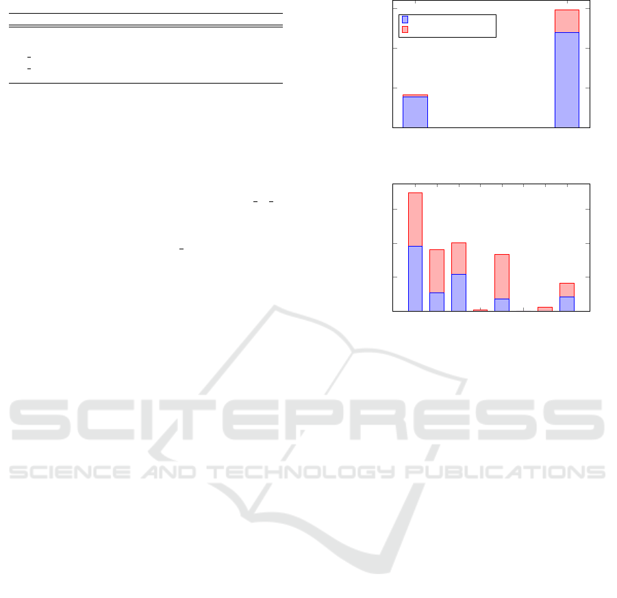
Table 2: Sliding Window results sim. data.

Mode Correctness 6 month Correctness 2 years Correctness

1D 81.97% 75.67% 78.82%

2D 92.84% 80.4% 86.62%

3D 1 23.48% 77.47% 62.22%

3D 2 11.88% 60.85% 36.37%

4D 0% 0% 0%

5.1.1 Sliding Window

Applying the different sliding window variants to the

simulated benchmark data sets produces prediction

results as depicted in Table 2. The best results are pro-

vided by the 2D approach that uses the hour of day

classiﬁer and the weekday classiﬁer. It is able to pre-

dict about 86% of the activity location pairs correctly.

The prediction quality of the 3D x and the 4D appro-

aches decreases, since the number of training context

tuples does not saturate the underlying histogram ade-

quately.

That partially explains the bad results of applying

the sliding window variants on the real world data sets

as shown in Table 3. The best results are provided

by the 1D approach with the least number of spanned

equivalence classes, but even then the prediction qua-

lity is too inaccurate to use it for the activity location

prediction in real world scenarios.

We tested the sliding window approach with diffe-

rent window lengths, but since the number of context

tuples in the real world data set was too low to satu-

rate the histogram adequately, we used the full range

of context tuples.

On the synthetic data set we found a global opti-

mum for the sliding window value at half of the con-

sidered period. So for the 6 month data set it is suf-

ﬁcient to consider the last 3 months of context tuples

while on the 2 years data set 12 months must be con-

sidered.

5.1.2 Bayesian Network

The Bayesian approach shows a much better overall

performance on the simulated data as well as on the

real world data. By applying the Bayesian approach

on the simulated data we get a prediction quality of

over 80% (Figure 3) and on the real world data it is

still around 40% (Figure 4), if there is a reasonable

training set. Yet, a 100% prediction rate is not possi-

ble since there exist unique events in both, the training

data and the real world data.

The poor prediction results for the users D, F and

G show, that also the Bayesian approach has a mini-

mal requirement of training data sets that must be rea-

ched to ensure a feasible prediction quality. However,

overall the results are much better on small training

6 month 2 years

10,000

20,000

30,000

Benchmark Data

# Correct Predictions/ Prediction Requests

Correct Predictions

Prediction Requests

92.84%

80.40%

Figure 3: Bayesian benchmark results of the simulated data.

A B

D E F

2,000

4,000

6,000

Test Persons

# Correct Predictions/ Prediction Requests

54.75%

29.58%

53.76%

1.67%

21.77%

3.39%

0.00%

49.88%

Figure 4: Bayesian benchmark results of the real data.

sets than the sliding window approach and we do not

need to estimate parameters, as the sliding window

value in the histogram based approach or the learning

parameters in the multilayer perceptron approach.

If we consider only the users A, B, C, E and F in

the real world data set (Figure 4), which provide 98%

of the tracking points the overall prediction quality is

41.95%. So given a reasonable time period to train

the Bayesian network it beats the sliding window ap-

proach.

5.1.3 The Multilayer Perceptron

A problem of the multilayer perceptron approach is

to ﬁnd suitable learning parameters that optimize the

prediction quality as best as possible. We need to de-

termine a suitable learning rate and an epoch value.

The epoch represents the number of training iterati-

ons, while the learning rate determines the inﬂuence

of each training iteration. Given a training set T of

size k ∈ N and an epoch l ∈ N : l > k we randomly

pick a value in T l times and train the system. With

l > k we ensure that every value in T is potentially

used for training and we do not restrict the training

set to a smaller subset.

In the following we use two different values for l:

10 · k and 100 · k for the simulation and the real world

data, respectively. In this way every single context

tuple has the chance of being used ten times in the

ﬁrst variant and a hundred times in the second variant.

Context-based User Activity Prediction for Mobility Planning

573

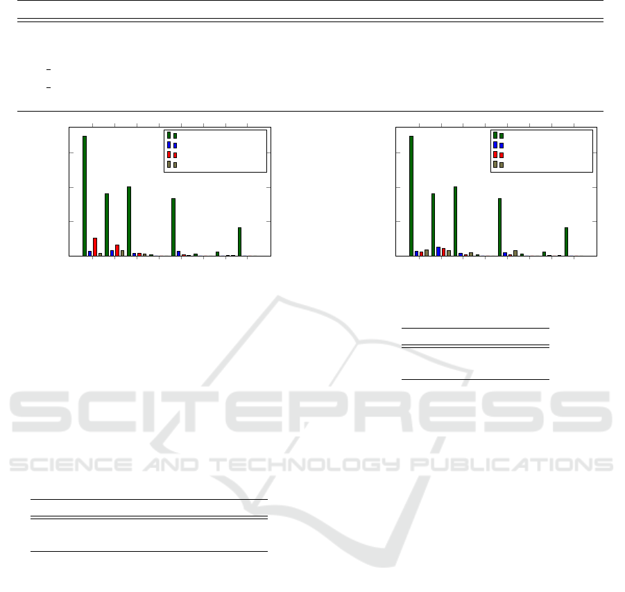
Table 3: Sliding Window results real world data.

Mode A B C D E F G H Overall

1D 2.17% 0.55% 1.49% 1.67% 0.66% 2.54% 1.35% 1.51% 1.49%

2D 0.30% 0.06% 0.45% 1.67% 0.12% 2.54% 1.35% 0.54% 0.88%

3D 1 0% 0% 0.05% 0% 0% 2.54% 1.35% 0% 0.49%

3D 2 0.01% 0% 0.07% 0% 0% 2.54% 1.35% 0.54% 0.56%

4D 0% 0% 0.05% 1.67% 0.03% 2.54% 1.35% 0% 0.71%

A B

D E F

2,000

4,000

6,000

Test Persons

# Correct Predictions/ Prediction Requests

Prediction Requests

Learning Rate 0.05

Learning Rate 0.2

Learning Rate 0.4

Figure 5: Multilayer perceptron user data ×10 epoch.

Nevertheless, there is still the problem of ﬁnding

a suitable learning rate e ∈ (0, 1]. If it is chosen too

big we overstep the minimum that optimizes the result

and if we choose it to small it needs too many itera-

tion to reach the minimum. Thus ﬁnding a suitable

learning rate is best done by comparing a number of

aspirants.

An overview of the overall correctness using the

synthetic benchmark data for different epoch values

and learning rates is given in Table 4.

Table 4: MLP benchmark results of the simulated data.

learning rate 0.05 0.2 0.4

×10 3.3% 6% 3%

×100 4.5% 2.25% 4.63%

The best results for the 10 ∗ k data sets is provided

by a learning rate of 0.2, while for an epoch of 100 ∗ k

the best results are provided by a learning rate of 0.4.

The benchmark results for applying the multilayer

perceptron approach on the real world data is depicted

in the Figures 5 and 6. The ﬁrst shows the result for

an epoch of 10 times the number of training context

tuples and the second ﬁgure shows the results for 100

times the number of training context tuples. Both re-

sults are very poor and similar to the results of the

synthetic benchmark data.

The prediction quality strongly depends on the

correct choice of the parameters. Thereby the choice

of the parameters depends both on each other and the

underlying training data. That means a good learning

rate for a certain epoch value is not necessarily a good

learning rate for another epoch value. Additionally a

good parameter pair for a certain training set doesn’t

A B

D E F

2,000

4,000

6,000

Test Persons

# Correct Predictions/ Prediction Requests

Prediction Requests

Learning Rate 0.05

Learning Rate 0.2

Learning Rate 0.4

Figure 6: Multilayer Perceptron user data ×100 epoch.

Table 5: Correctness of home and work location prediction.

Location Correctness

home 62.5%

work 37.5%

necessarily provide good results for another training

set.

To ensure good prediction results using the multi-

layer perceptron much more training data is necessary

than can be captured by a common user. This will re-

duce the inﬂuence of training parameters on the pre-

diction results.

5.2 Place Name Mapping

Regarding the benchmark data we can derive the cor-

rect home location of a person with a probability of

62.5%. The correct work location is still estimated

with a correctness of 37.5% (cf. Table 5). Especi-

ally the home and work location estimation of users

that provide only a low number of tracking points D,

F and G in Figure 2 is erroneous. Thereby for users

F, G the home location was assumed to be the work

location.

If we consider only those users that provide a rea-

sonable number of tracking points we get success ra-

tes of 100% for the home location and still 62.5% for

the work location.

ICAART 2019 - 11th International Conference on Agents and Artiﬁcial Intelligence

574

6 CONCLUSION

In this paper we examined the question whether it is

possible to automatically plan a trip by deriving the

departure location, the arrival location and the arrival

or departure time from a user’s device context.

We reduced the problem of providing travel as-

sistance to the problem of predicting the activity and

location of a person given a certain time and date.

We tested three different approaches providing

activity/location predictions and compared them to

each other. The best results are provided by the Bay-

esian network based approach that was able to make

correct predictions in about 40% of the cases. It also

provides the best results with respect to the training

speed, since it has the best prediction quality even on

a small number of context tuples. A system based on

the Bayesian approach can be used after a short initi-

alization and training period.

We further introduced an approach to identify the

home and work location of a person based on rating

functions. We were able to estimate the home location

in about 62.5% of the cases and the work location in

about 37.5% of the cases.

For future work we plan to tweak the multilayer

perceptron by testing different architectures. Eva-

luation results suggest that certain architectures that

work good on a small number of context tuples fail

on a great number of context tuples and vicit versa. A

combination of different architectures chosen with re-

spect to the number of available context tuples could

solve the problem.

REFERENCES

Ambite, J. L., Barish, G., Knoblock, C. A., Muslea, M., Oh,

J., and Minton, S. (2002). Getting from here to there:

Interactive planning and agent execution for optimi-

zing travel. In Proceedings of the Eighteenth Nati-

onal Conference on Artiﬁcial Intelligence, July 28 -

August 1, 2002, Edmonton, Alberta, Canada., pages

862–869.

Ashbrook, D. and Starner, T. (2002). Learning signiﬁcant

locations and predicting user movement with GPS. In

6th International Symposium on Wearable Computers

(ISWC 2002), 7-10 October 2002, Seattle, WA, USA,

pages 101–108.

Bhattacharya, S., Kukkonen, J., Nurmi, P., and Flor

een, P.

(2008). Serpens: a tool for semantically enriched loca-

tion information on personal devices. In 3rd Interna-

tional ICST Conference on Body Area Networks, BO-

DYNETS 2008, Tempe, Arizona, USA, March 13-15,

2008, page 30.

Coyle, L. and Cunningham, P. (2003). Exploiting re-

ranking information in a case-based personal travel

assistent. In Workshop on Mixed-Initiative Case-

Based Reasoning at the 5th International Conference

on Case-Based Reasoning, pages 11–20.

Dillenburg, J., Wolfson, O., and Nelson, P. (2002). The

Intelligent Travel Assistant.

Foundation for Intelligent Physical Agents (2001). FIPA

personal travel assistance speciﬁcation. Draft Speciﬁ-

cation XC00080B, FIPA.

Kim, S. and Cho, S. (2014). Predicting Destinations with

Smartphone Log using Trajectory-based HMMs. MO-

BILITY 2014, The Fourth International Conference on

Mobile Services, Resources, and Users, (c):6–11.

Mozer, M. C. (1998). The neural network house: An envi-

ronment that adapts to its inhabitants. American As-

sociation for Artiﬁcial Intelligence Spring Symposium

on Intelligent Environments, pages 110–114.

Nazerfard, E. and Cook, D. J. (2013). Using bayesian net-

works for daily activity prediction. In Plan, Activity,

and Intent Recognition, Papers from the 2013 AAAI

Workshop, Bellevue, Washington, USA, July 15, 2013.

Tran, L., Catasta, M., McDowell, L. K., and Aberer, K.

(2012). Next Place Prediction using Mobile Data.

Proceedings of the Mobile Data Challenge Workshop

(MDC 2012).

Wang, J. (2012). Periodicity Based Next Place Prediction.

Nokia Mobile Data Challenge 2012.

Waszkiewicz, P., Cunningham, P., and Byrne, C. (1999).

Case-based User Proﬁling in a Personal Travel Assis-

tant, pages 323–325. Springer Vienna, Vienna.

Wolf, J., Guensler, R., and Bachman, W. (2001). Elimi-

nation of the travel diary: Experiment to derive trip

purpose from global positioning system travel data.

Transportation Research Record, 1768(1):125–134.

Context-based User Activity Prediction for Mobility Planning

575