Physically-based Thermal Simulation of Large Scenes for Infrared

Imaging

B. Kottler, E. Burkard, D. Bulatov and L. Harak

Department of Scene Analysis, Fraunhofer Institute of Optronics, System Technologies and Image Exploitation (IOSB),

76275 Ettlingen, Germany

Keywords:

Physics-Based, Thermal Infrared, Heat Simulation, Heat Transfer Modeling, Finite Volume Method.

Abstract:

Rendering large scenes in the thermal infrared spectrum requires the knowledge of the surface temperature

distribution. We developed a workﬂow starting from raw airborne sensor data yielding to a physically-based

thermal simulation, which can be used for rendering in the infrared spectrum. The workﬂow consists of four

steps: material classiﬁcation, mesh generation, material parameter assignment, and thermal simulation. This

paper concerns the heat transfer simulation of large scenes. Our thermal model includes the heat transfer types

radiation, convection, and conduction in three dimensions within the object and with its environment, i.e. sun

and sky in particular. We show that our model can be solved by ﬁnite volume method and it shows good

agreement with experimental data of the CUBI object. We demonstrate our workﬂow for sensor data from

the City of Melville and produce reasonable results compared to infrared sensor data. For the large scene, the

temperature simulation ﬁnished in appropriate time of 252 sec. for ﬁve day-night cycles.

1 INTRODUCTION AND

PREVIOUS WORK

1.1 Motivation

Thermal simulation of large scenes is essential when

it comes to applications like meteorology, assessment

of atmospheric pollution, camouﬂage evaluation in

the military applications or detection of urban heat is-

lands and corresponding heat radiation for city plan-

ners. All these applications and especially the last one

have a strong dynamic component, since to the same

extent as augmentation of both the global earth tem-

perature rises, so does urbanization degree.

From the point of view of a city planner, whose

job is to respond to the needs of the later generations

without putting upside down the infrastructure needed

for the current one, the ability to render large three-

dimensional scenes in thermal infrared wavelength

spectrum is a very interesting aspect. In which dis-

tances along the roads should the trees be planted and

which kinds of trees should actually be used to reduce

the heat radiation to an acceptable amount? Which

heights and roof materials for the public buildings are

least susceptible to the appearance of urban heat is-

lands? Fast and reliable scene rendering in thermal

infrared allows assessing the long-term energy bal-

ance for these scenarios. The temperature of the sur-

face should be ideally modeled as a function of the

current atmospheric condition, surface geometry and

material composition, socio-economic situation, and

many others. Of course, a city planner cannot start

from scratch, but must deal with the existing realities,

or initial conditions. For a more precise simulation of

temporal development of the surface temperature and

subsequent thermal rendering, the main requirement

is to know as much as possible about the surface. Here

it is often not enough to use the existing geographical

data, because they may be obsolete or just lack some

relevant information, such as building roof materials

and roof forms.

To be able to free ourselves from too many input

requirements (accurate 3D models, numerous tem-

perature measurements), we are currently designing

an end-to-end pipeline starting at raw airborne sen-

sor data and yielding semantic and three-dimensional

environments rendered in thermal infrared. The fo-

cus of this paper will concern the simulation of the

surface temperature of large scenes. This may not

only be used directly in many applications but also

is basic for thermal rendering, i.e., determining the

heat radiance since every object having a tempera-

ture above absolute zero radiates at infrared wave-

lengths. The reason to utilize the airborne data is that

Kottler, B., Burkard, E., Bulatov, D. and Haraké, L.

Physically-based Thermal Simulation of Large Scenes for Infrared Imaging.

DOI: 10.5220/0007351400530064

In Proceedings of the 14th International Joint Conference on Computer Vision, Imaging and Computer Graphics Theory and Applications (VISIGRAPP 2019), pages 53-64

ISBN: 978-989-758-354-4

large parts of the scene are captured and the measure-

ments of geometry and material classiﬁcation are ac-

tual. From these measurements, there are plenty of

previous work achieved on accurate 3D city model-

ing and material classiﬁcation (Bulatov et al., 2014;

Xiong et al., 2014). The ﬁrst reason for producing

semantic scenes is that land-cover classes and mate-

rial classes are strongly correlated, e.g. within one

building, roofs consist of few materials, trees can be

represented by generic models. Otherwise assigning

materials to single roof polygons making up the scene

and ﬁguring out the emitting properties of these ma-

terials are two tedious procedures. The second reason

is that once these models are available, further im-

portant data, such as material composition of building

walls or analysis of socio-economic developments are

easier to integrate. A particular challenge for the ge-

ometry component of the above module is the com-

plexity of the underlying scene. Besides, shadow

cast is a crucial component for surface temperature,

which cannot be employed in 2D case (Dewan and

Corner, 2014). Finally, to provide an accurate ground

truth measurement in closest-range three-dimensional

scenarios, which are appropriate for detecting urban

heat islands, among others, an efﬁcient rendering rou-

tine can replace numerous punctual measurements of

temperatures and provide a glance into the future by

means of simulation. The complexity of the prob-

lem is the reason why there are only a few publica-

tions focused on simulation of surface temperature in

larger three-dimensional environments, as we will see

in the remainder of this section. Also, we will see that

(Xiong et al., 2016) is the most similar contribution to

our work, however, there are still several differences

and improvements it is worth being focused on.

1.2 Previous Approaches

We start our short literature review by 2D-based ap-

proaches. Essentially, convection and emission equa-

tions are retrieved from land-cover/material classi-

ﬁcation results (Bartos and Stein, 2015; Feng and

Myint, 2016; Dewan and Corner, 2014). Three-

dimensional scene elements are treated by unfold-

ing; hence, effects of shadow cast remain unconsid-

ered. However, for close-range applications around

selected monuments, the surrounding 3D terrain

(heights of the trees and buildings) must not be ne-

glected and thus the challenge is to combine the auto-

matic urban terrain reconstruction and thermal simu-

lation. A well-established software MuSES, designed

for the US army, is introduced in (Johnson et al.,

1998). In particular, it shows how the level of au-

tomatization in thermal simulation was increased with

respect to the previous system. The remaining inter-

active parts were on the one hand uploading the 3D

geometry and assigning material properties, and on

the other hand, quality control since the system was

presumable used for camouﬂage and deception. It be-

comes clear that an automatic creation of 3D mod-

els assigned with material properties is tempting for

a more rapid progress in the ﬁeld. The authors of

(Lagouarde et al., 2010) are more interested in mea-

suring temperatures from different viewing directions

since it correlated with radiation emitted by an en-

semble of structure. In the ﬁrst part of their work,

they assess directional anisotropy that is the differ-

ence between the directional and the nadir tempera-

tures. In the second part of the work, the model at a

given direction is rendered and the aggregated direc-

tional temperature at a given pixel in obtained using

the classes and the raw values for the surface temper-

ature from the ﬁrst step. While the 3D models were

provided from the public sources, the authors only

made a difference between six conﬁgurations, that is

two light settings (sunlit or shaded) and the three land-

cover classes (roof, wall, and soil with materials as-

signed more or less arbitrarily). Performing the three-

dimensional aggregation of temperatures is another

critical generalization of their method. The advanced

treatment of shadows is described in (Poglio et al.,

2002). The authors adaptively subdivide the triangles

in illuminated and shaded ones, ensuring that the new

triangles are not degenerated. As for development of

the simulated scene over time, they refer to (John-

son et al., 1998). A summary of the physics of heat

transport in large scenes can be found in (Mar

echal

et al., 2010). In their voxel-based approach, a method

for simulating realistic winter appearance based on a

physical simulated temperature distribution for alpine

regions is presented. For us this paper gives a good

overview about components of our simulation.

Most similar to our contribution is (Xiong et al.,

2016). From raw meshes, classiﬁcation of triangles

into ground, vegetation, building wall and building

roof takes place using simple 3D-based features (ele-

vation, planarity, and horizontality) and Markov Ran-

dom Fields. In the next steps, the portions of the mesh

corresponding to buildings are modeled as water-tight

multi-planar structure while the remaining elevated

portions of the mesh are ignored. For every mesh

element, heat balance equation comprising terms for

radiation, conduction, and convection is solved. The

shadows are taken into account as well in the radiation

term. This pioneering work can be questioned in two

aspects. First, the raw meshes were created from im-

ages by means of structure from motion procedures.

However, the images were not considered for assign-

GRAPP 2019 - 14th International Conference on Computer Graphics Theory and Applications

ing material properties to surface triangles. The sec-

ond problem is that the vegetation was not considered

even though presence of trees is very valuable for re-

ducing the urban heat.

1.3 Contributions

Our improvements will include land-cover classiﬁ-

cation from combined image- and point-based fea-

tures. From the image based classiﬁcation result,

we triangulate the terrain using Restricted Top-Down

Quadree Triangulation (Pajarola, 2002). The triangu-

lated terrain has three important properties: memory

efﬁciency, accuracy, and consistence.

To this terrain mesh, we add the building mod-

els. For this contribution, we will use the terms land-

cover and material classiﬁcation synonymous, assum-

ing, for example, that the building roofs and walls

are comprised by two uniform materials. Contribu-

tions achieving a more detailed subdivision of build-

ing roofs into materials using multi-spectral and high-

resolution images exist in the literature (Ilehag et al.,

2018) and thus our approach can be easily extended.

Besides, we detect high vegetation and add trees to

the mesh as well, currently modeled in the shape of

forest boxes, i.e. trees standing close to each other

are merged and single trees are disregarded. Further-

more, we are able to take shadows into account as

the simulation is performed on a surface embedded in

the 3-dimensional space and thus includes occlusion

analyses.

A physical approach was chosen to calculate the

surface temperatures with the heat equation. This is

a partial differential equation, i.e. it includes spatial

and temporal derivations. For the temporal deriva-

tions, the forward Euler integration was used. The

spatial derivations were discretized with a ﬁnite vol-

ume method. For this purpose, the simulation area

is divided into ﬁnite volumes and the ﬂows on the

boundaries of the volumes are evaluated. We will con-

sider ten classes in total and for each of these classes,

we derive the necessary coefﬁcients from the litera-

ture.

In this paper, we propose a framework for sim-

ulating realistic temperature distributions for large

sceneries. This is the core aspect of a complex work-

ﬂow from sensor data to semantic urban terrain mod-

els rendered in thermal spectrum.

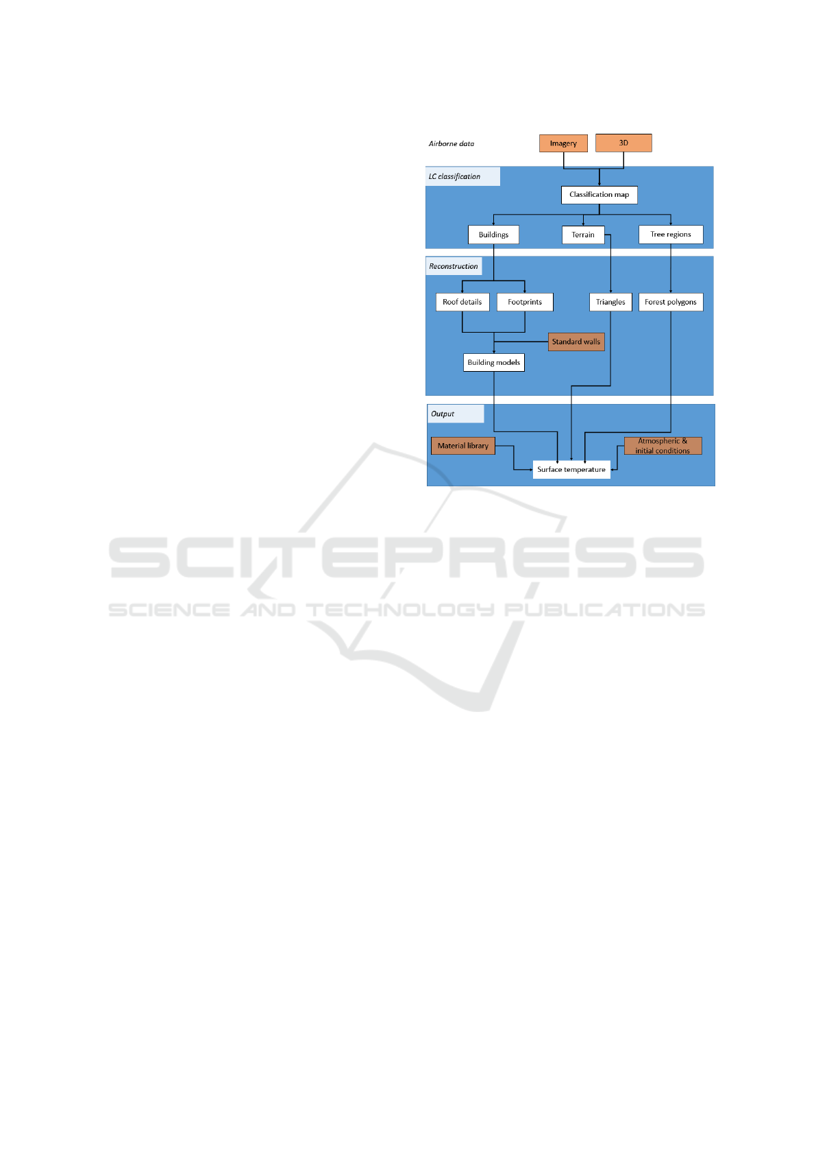
2 PRELIMINARIES

Since the focus of this paper concerns the temperature

simulation step of the pipeline, or the bottom block of

Figure 1: Pipeline – From Sensor to Surface Temperature.

Figure 1, we decided to give a short summary of the

physical background necessary for thermal simulation

and how it states the basis for infrared rendering, as

well as the preceding steps leading from raw airborne

data to a semantic 3D representation of the scene.

2.1 Infrared Rendering and Physical

Background of Thermal Flow

Starting with the Kajiya’s well-known rendering

equation, cp. (Kajiya, 1986),

L(x,

ω) = L

(x,

ω) + L

(x,

ω), (1)

with the total radiance L(x,

ω) from surface point x

in direction

ω which consists of the emitted radiance

and the reﬂected radiance from the upper hemi-

sphere of the surface L

, we have to take into account

the temperature dependence of the emissive radiation

term L

if regarding the thermal spectrum for render-

ing,

(x,

ω) = L

(x,

ω,T ), (2)

where T is the surface temperature at point x. In order

to evaluate this equation and render an arbitrary scene

in the infrared spectrum, one has to know the sur-

face temperature at every observed point in the scene.

However, temperature is not a property as color or

texture, but depends on the environment, time of the

day, physical material parameters, temperature his-

tory, and so on. Determining the surface temperature

Physically-based Thermal Simulation of Large Scenes for Infrared Imaging

of a scene at a speciﬁc point in time requires the sim-

ulation of heat transfer.

In general, heat transfer follows the ﬁrst law of

thermodynamics where we will consider constant vol-

umes,

= Q (3)

with the mass m, the speciﬁc heat capacity C

at con-

stant volume, the temperature T and the heat trans-

fer rate Q per unit area (Lienhard IV and Lienhard V,

2011). This rate is compound by the three modes of

heat transfer: radiation, conduction and convection.

For the sake of completeness, it shall be pointed out

that heat can also be chemically stored in the form

of latent heat caused by phase change, e.g. vaporiza-

tion. However, this will not be included in the thermal

model presented in this paper.

Heat conduction takes place predominantly within

solids and ﬂuids, and the conductive heat transfer fol-

lows Fourier’s law,

= K ∆T (4)

with the thermal conductivity K. Convection involves

the surrounding medium, e.g. the air in an urban

area. Free convection describes the phenomenom of

a medium being heated or cooled by a surface and

therefore starting to move. Forced convection refers

to an already moving medium, e.g. due to wind, ex-

changing heat with a surface. The convective heat

transfer depends on the difference between the sur-

face temperature T and the surrounding mediums’

temperature T

medium

∂T

∂t

∝ T − T

medium

. (5)

Regarding radiative heat transfer, all matter with

a temperature greater than absolute zero emits ther-

mal radiation. For a blackbody, which is deﬁned by

absorption end re-emission of all incoming light, the

radiation power follows the Stefan-Boltzmann law,

P = σT

with the Stefan-Boltzmann constant σ, and

the temperature T (Siegel and Howell, 1992). With

the so-called grey-body approach, the actual radiative

power is given by a constant fraction of a blackbodys’

radiative power, deﬁned by the emissivity ε ∈ [0,1],

where ε = 1 equals a blackbody. In estimating the bal-

ance heat transfer in a scene with several objects, one

has to model the heat radiation of each object and tak-

ing into account the mutual visibility. This is where

the 3D geometry of the scene becomes indispensable.

With sun and sky as main participants, the challenge

is to efﬁciently perform shadow analysis.

Figure 2 shows an overview of the types of the

modeled thermal phenomena.

Figure 2: Overview of the considered physical phenomena

in the thermal simulation.

2.2 From Sensor Data to Semantic

Surface Representation

The semantic reconstruction and material classiﬁca-

tion are important preprocessing steps, since the heat

simulation depends strongly on the material proper-

ties and geometry, as mentioned above.

We assume the availability of the elevation data,

sampled into DSM (Digital Surface Model). Com-

bining image and elevation data, land-cover classes

are obtained. Hereby, the building class is particu-

larly important for the subsequent 3D modeling step,

since buildings as man-made objects are heated or

cooled from the inside, or roof materials are gener-

ally different. Other important classes are: bare soil,

grass, tree, water and road. Various approaches ex-

ist for land-cover classiﬁcation. We are interested

in ones which need only a few training patches and

features. Therefore, we opted for a conventional ap-

proach based on Random Forests classiﬁer (Breiman,

2001). As image-based features, we took the chan-

nels of the multispectral image, vegetation and water

indices. As elevation-based features, we considered

relative elevation, whereby a standard interpolation

procedure was chosen to reconstruct the ground, as

well as the planarity measure (Gross and Th

onnessen,

2006). Training patches were sampled interactively.

After building detection, (Bulatov et al., 2014) sug-

gest performing their delineation (for simpliﬁcation

of shapes), outlining and roof detail reconstruction.

However, building models resulting from such a data-

driven approach are not water-tight, causing problems

for the simulations. Therefore and because in our

data set, the buildings are not too high, for this work,

we decided to use the freely available shapeﬁle with

building outlines and to model every building as a

prismatic structure with elevation retrieved from sen-

sor data. Building walls are modeled as vertical trape-

zoids by projecting the endpoints of border- or step-

GRAPP 2019 - 14th International Conference on Computer Graphics Theory and Applications

edges of the roof to the ground. For the tree regions,

we will concentrate on large forest regions. They are

represented as forest boxes and allow to model huge

forest areas by at most several dozens of polygons

(Decaudin and Neyret, 2004; H

aufel et al., 2017). The

last data preparation step concerns meshing of the ter-

rain. Starting at the classiﬁcation result, we wish to

assign a class to every triangle. Therefore, after sev-

eral morphological operations allowing to suppress

too small regions, we consider a canonical rectangu-

lar grid along the axes x and y. Tracing one diagonal

of each rectangle in the grid as well as assigning the

ground values of vertices as z coordinates results in a

coarse triangle mesh. In the initial mesh, those trian-

gle with either elevation or class discontinuities can

be subdivided along their symmetry axis into a pair of

smaller triangles. In order to avoid cracks in the ﬁ-

nal surface (that result if a 2D mesh vertex is an inner

point of an edge, because the corresponding 3D point

is not necessarily incident with the an edge connect-

ing the 3D endpoints of this edge), adjacent triangles

must be subdivided as well and, sometimes, new ver-

tices must be inserted. This approach was referred in

(Pajarola, 2002) as restricted (top-down) quadtree tri-

angulation (RQT or RTDQT) and was implemented

in this work.

3 MODELING THERMAL

TRANSFER

In this section, we present our architecture for sim-

ulating thermal transfers for large sceneries, whose

geometry is determined by a surface model. First,

the data representation and our simulation basis re-

ferred to as surface volume are introduced. Further-

more, we give an overview of the considered physical

parameters of one surface volume element and the en-

vironmental model as well as the core equation for the

implementation. Finally, a mathematical description

of the considered physical modes of heat transfer is

given.

3.1 Data Representation and Model

Principle

Surface Volume Model: The basis of the simula-

tion is the heat equation, which describes the distri-

bution of heat in a given volume over time. For this,

we extend the surface model of the scene to a surface

volume by giving the surface a thickness.

There are three types of heat propagation in this

volume: the heat can be propagated by conduction

within the volume, there is a heat exchange with the

outside world and heat exchange with the inside of the

body. Mathematically, the thermal conduction in the

surface volume can be described with the heat equa-

tion and suitable boundary conditions:

∂T

∂t

= K∆T in the interior, (6)

T = T

Core

on the inner surface, (7)

∇T · n = Q on the outer surface, (8)

where n is the outer normal of the wall surface and

the thermal conductivity K of the material. In this

model, the inner side of the surface volume interacts

only with the inner body, which has an internal tem-

perature T

Core

assumed to be constant. The core tem-

perature can be used to model socio-economic condi-

tions, such as heated buildings. The outer side inter-

acts with the outer world, where the total heat ﬂow is

denoted with Q.

For solving this partial differential equation a ﬁ-

nite volume method in 3D is implemented. For this

purpose, the surface is discretized with a coarse trian-

gular mesh, which was given a thickness. The ﬁnite

volume method is based on balancing the thermal en-

ergy ﬂux of the triangular prisms.

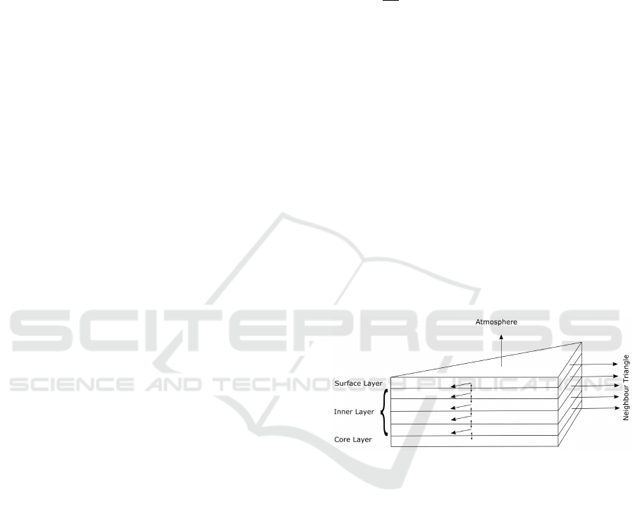
Figure 3: Principle of surface volume discretization.

Model of Geometry and Materials: The basis of

the simulation is a triangulated surface mesh repre-

senting the geometry of the scene in which the third

dimension is implicitly treated. The surface volume

model consists of N layers, that means for each trian-

gle overall 2+N temperature values have to be stored:

the surface temperature, N temperature values for ev-

ery layer, and the core temperature (see Figure 3).

Furthermore, every triangle is assumed to consist

of one speciﬁc material class, which implies a set of

parameters representing the physical properties ac-

cording to Table 1. The parameters can be divided

into material properties and environmental properties,

the latter ones depend not only on the material but on

environmental model and correspond not necessarily

to a physical equivalent.

Physically-based Thermal Simulation of Large Scenes for Infrared Imaging

Table 1: Overview of Parameters.

Material Properties Symbol

Albedo α

Emissivity ε

Density ρ

Speciﬁc heat C

Thermal conductivity K

Thickness of the layers d

,...d

Environmental Properties

Core temperature T

Core

Free convection h

Forced convection h

Wind velocity v

wind

Air temperature T

air

Relative humidity r

Discretization of the Inner Model: The discretiza-

tion of the model is similar to (Bartos and Stein, 2015)

with the difference that we set the parameters using a

database and do not need to be ﬁtted. The model of

the inner temperature for N layers leads to a system

of N +1 coupled differential equations, describing the

temperature along the proﬁle of the surface volume.

For the ﬁrst inner layer we have the equation

∂T

∂t

− 2T

+ T

) + K∆T

, (9)

for layers with the index i = 1,...,N −1, we have

∂T

∂t

i−1

− 2T

+ T

i+1

) + K∆T

, (10)

and for the last inner layer we have

∂T

∂t

N−1

− 2T

+ T

Core

) + K∆T

. (11)

Model of the Environment: The model for the en-

vironment consists of a small set of functions de-

scribing the time course of the weather. The weather

parameters taken into account are the air tempera-

ture T

Air

(t) ∈ R and relative humidity r(t) ∈ [0, 100],

which can be varied between triangles. Furthermore,

the cloud cover is described by C(t) ∈ [0,1], where

0 stands for cloud-free sky and 1 for a dense cloud

cover. The atmospheric damping is summarized by

the factor I

(t) ∈ [0.3,0.8], which is called clearness

index. It is deﬁned by I

(t) = 0.8 − 0.5C(t), cf.

(Mar

echal et al., 2010). The environmental param-

eters have to be precalculated from weather data or

speciﬁed by the user.

Temporal Discretization: For every triangle of the

scene the current temperature, material parameters are

stored. The time discretization is performed using a

forward Euler integration scheme. Let ∆t denote the

time step for integration of triangle i. At every time-

step n, the total ﬂux Q

is computed as the sum of all

heat ﬂuxes, hence the new temperature is computed

n+1

= T

∆t, (12)

where d

denotes the thickness of the layer corre-

sponding to the triangle i. The parameter ∆t is cho-

sen after a stiffness analysis of the linear system. Nu-

merical experiments have shown that a time step of

∆t = 30s leads to stable results and records the time-

dependent weather phenomena with a good accuracy.

3.2 Physical Modeling of Thermal

Flows

In the following, we present the modeling of thermal

ﬂuxes, describing the physical phenomena mentioned

in Section 2.1 and some details of the numerical im-

plementation.

The thermal change of a surface volume is calcu-

lated using the heat equation

ρd

∂T

∂t

= A + I +D + R + S = Q, (13)

where A describes the convective thermal exchange

with the surrounding air, I describes the inner model

of the surface, D describes the conductive thermal ex-

change with neighboring triangles, R describes the ra-

diative thermal exchange with the sky, and S describes

the thermal ﬂow through direct sunlight. The total

ﬂux is denoted with Q. The following deals with the

modeling of these ﬂuxes.

3.2.1 Convective Thermal Exchange

The thermal exchange between the surface and the

surrounding air is divided into free convection and

forced convection whereas we choose a linear model.

Let h

denote the coefﬁcient for free convection and

the coefﬁcient for forced convection, v

wind

the

wind speed, and T

Air

the temperature of the air. Then

the heat ﬂux between a surface triangle and the air

can be described by Newton’s law of cooling for free

convection and a linear model for forced convection

A = (h

+ h

· v

wind

)(T

Air

− T

). (14)

3.2.2 Conductive Thermal Exchange with the

Inner Model

Heat conduction dominantly depends on the materials

thermal conductivity. Assuming only homogeneous

GRAPP 2019 - 14th International Conference on Computer Graphics Theory and Applications

media and considering only temperature ranges typi-

cal for urban sceneries, the thermal conductivity can

be assumed constant (Lienhard IV and Lienhard V,

2011). Regarding one-dimensional ﬂow, the surface

temperature is coupled to the inner model with the

connection

I =

− T

), (15)

where d

is the discretization parameter deﬁning the

surface layers’ thickness.

3.2.3 Conductive Thermal Exchange Along the

Surface

In addition to conduction into the interior of the body,

there is also conduction along the surface. It is calcu-

lated with a discretization of the Laplace operator in

D = K∆T

. (16)

The discretization of the gradient along the surface is

done with a ﬁnite volume method, where for every

face of the triangle the heat ﬂux of the neighboring

triangle is calculated. The total ﬂux for a triangle i

with the area A

is then given by

(∆T )

≈

∑

j∈N

i j

(∇T )

i j

· n

i j

. (17)

where N denotes the set of neighboring triangles of

triangle i, (∇T )

i j

the ﬂux, n

i j

the outer normal of the

edge between triangle i and triangle j, and L

i j

the

length of that edge.

3.2.4 Radiative Thermal Exchange with the Sky

In our model, we assume that a surface triangle can be

either oriented to the sky and exchange thermal radia-

tion, or oriented to another surface triangle, which has

a similar temperature, so the thermal radiation can be

neglected.

In a preprocessing step using OpenGL renderings

of the scene with different angles, the visibility of the

surface is determined. A rendering is done in two

steps. First, the scene is rendered from the perspective

of sky and the depth information is stored for each vis-

ible object. Then the scene is rendered again, where

for each pixel the depth information is used to deter-

mine whether it is visible to the sky. If this is the case,

the pixel store the index of the corresponding triangle.

After a histogram analysis, the portion of the surface

of each triangle that is not occluded by other triangles

is determined. The visibility of the surface from the

viewpoint of the sky is then deﬁned as the mean of all

angles and denoted by the parameter γ

Sky

∈ [0,1].

The temperature of the sky depends on the temper-

ature of the air, the dew point temperature for a cloud-

less sky and the time of day denoted by h(t) ∈ [0, 24].

The dew point temperature T

is approximated by

the Magnus approximation with the air temperature

Air

and relative humidity r through saturation vapour

pressure (SVP) and vapour pressure (VP), c.f (Son-

ntag, 1990)

SVP(t) = 6.1078 · 10

a·T

Air

(b+T

Air

)

, (18)

VP(t) =

100

· SVP, (19)

(t) = b ·

v(t)

a − v(t)

, (20)

where v(t) = log



V P(t)

6.1078



and



a = 7.5, b = 237.3 for T

Air

≥ 0,

a = 7.6, b = 240.7 for T

Air

< 0.

(21)

As in (Mar

echal et al., 2010), the temperature of the

clear sky is approximated by

Sky

= T

Air

(t)



0.711 + 0.0056 T

(t)

+7.3 · 10

−5

(t)

+ 0.013cos

2πh(t)



(22)

The temperature of the clouds is calculated based on

the assumption that the air temperature drops 9.84

◦

and dew point temperature drops 1.82

◦

C per 1000 m

of altitude. Then, the height of the clouds can be esti-

mated by

cloud

= (T

Air

− T

)/(9.84 −1.82) · 1000. (23)

The following equation is used to estimate the clouds’

temperature:

cloud

= −0.00182 · H

cloud

+ T

. (24)

The total temperature of the cloudy sky is approxi-

mated with the weighted mean of the cloud tempera-

ture and clear sky temperature, thus

total

= C · T

cloud

+ (1 −C)T

sky

, (25)

where C denotes the cloud cover index.

The total thermal ﬂux between a given trian-

gle and the cloudy sky is calculated by the Stefan-

Boltzmann law

R = εσγ

Sky

total

− T

), (26)

where ε denotes the emissivity of the material of the

triangle.

Physically-based Thermal Simulation of Large Scenes for Infrared Imaging

3.2.5 Thermal Heating by Direct Sunlight

The contribution of direct sunlight is the main source

of heat energy and therefore a critical part of the sim-

ulation.

The total amount of solar heat energy received by

a triangle depends on the total solar irradiation, which

varies during the year because of the eccentricity of

earth’s orbit, the orientation of the triangle to the sun,

atmospheric inﬂuences, and whether the triangle is

actually irradiated by the sun or shaded.

The solar irradiation outside of the atmosphere for

a surface directly faced to the sun can be approxi-

mated by

total

= 1367(1 + 0.033 cos(2πn/365)),

where n denotes the day of year, cf. (Mar

echal et al.,

2010). The fraction of the area facing the sun is cal-

culated from the sun direction s and the normal of the

surface n

by cos(ϕ) = s · n

, where ϕ denotes the an-

gle between the sun ray and surface normal. The solar

irradiance before atmospheric ﬁltering is given by

Sun

= E

total

· cos(ϕ).

The atmosphere absorbs solar radiation, which is

modeled by weighting the sun irradiance with the

clearness factor I

. Furthermore, a fraction of the ir-

radiance is not absorbed by the surface, but reﬂected

back. This effect is represented by the albedo of the

surface which depends on the color and material prop-

erty of the triangle, yielding to the solar irradiance

S = (1 − α)I

Sun

cos(θ), (27)

where θ is the sun’s elevation angle. If the triangle is

actually illuminated by the sun or occluded by other

triangles is stated by a factor γ

Sun

∈ {0, 1} which is

determined using an OpenGL rendering of the scene

analogous to 3.2.4. More precisely, an index image of

the scene from the viewpoint of the sun is rendered,

then γ

Sun

is set to 1 if the triangle is visible on the

rendered picture or 0 otherwise. This allows to deal

with thermal shadows in the simulation. In summary,

the solar irradiation on the surface is given by

S = (1 − α)I

Sun

cos(θ)γ

Sun

. (28)

4 RESULTS

In this section, the results for two data sets are pre-

sented. The method was implemented in MATLAB

with the parallel processing toolbox on an Intel(R) I7-

8700 3.19GHz CPU with 32GB RAM and NVIDIA

GeForce GTX 1080 GPU. The ﬁrst data set represents

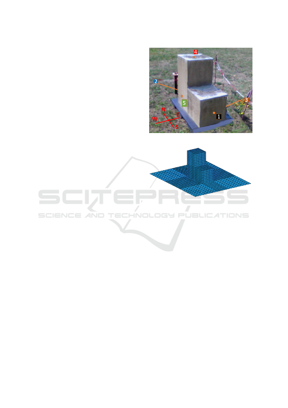
Figure 4: CUBI in Ettlingen with ﬁve thermistors (south,

north, east, top, west).

Figure 5: Watertight CUBI and Ground mesh with 2816

triangles.

a simple scene with known ground truth; hence it can

be used for validation. The second data set consists of

various sensor data of an urban area, so we used the

proposed four-step pipeline and compared the result

of the thermal simulation with a thermal image.

4.1 CUBI – Thermal Model Validation

CUBI is a simple geometrical object used in outdoor

experiments to collect data for testing and validation

of thermal models and infrared imaging. It has the

shape of a stair, like three compound cubes with an

edge length of 0.5m. For the validation of our ther-

mal model, we use the data of (Malaplate et al., 2007)

that include time series of different surface tempera-

ture acquired by thermistors in Ettlingen, Germany, in

May 2006. In Figure 4, the CUBI test object with the

positions of thermistors is shown.

Representing the geometry of CUBI and the

ground, a mesh with 2816 triangles was created, as

shown in Figure 5.

As material parameters for the CUBI as well as for

the ground, we use those for metal, retrieved from the

material database. For the inner model, 10 layers are

GRAPP 2019 - 14th International Conference on Computer Graphics Theory and Applications

Figure 6: Simpliﬁed air temperature curve used for simula-

tion.

used with a thickness of 0.1m.

We simulate a two-days cycle from 2006-05-11 to

2006-05-12 for the location of Ettlingen 48;56; 48 N

8;24;38E with a simpliﬁed air temperature curve

shown in Figure 6. We use the same air temperature

curve for both days with a minimum temperature of

◦

C at 4:00 am and a maximum temperature of 27

◦

at 3:00 pm.

Figure 7 shows the temperature distribution of the

CUBI at 1:00 pm. The thermal shadow of the CUBI

is recognizable by the blue color on the ground on the

right part of the picture. The heat conduction is also

clearly visible as color gradient at the shadow and at

the edges of surfaces, for those one surface is in the

shade and the other is illuminated by the sun.

In Figure 8 the collected and simulated data of the

thermistors is shown. Both curves show a good qual-

itative agreement: The order of the peaks is identical.

As expected, the eastern thermistor (brown/yellow)

reaches its maximum at about 10 o’clock and then

cools down in a similar way until evening, i.e. both

curves show a small hump. Also the maximum tem-

perature is about the same at 40

◦

C. The upper and

southern termistors (red and black) reach their max-

imum at about 12 o’clock, which corresponds to the

measured data, the temperature is only slightly over-

estimated in the simulation. Finally, the western ther-

mistor reaches its maximum in the evening, which

is slightly underestimated compared to the measured

data. The northern thermistor (blue) is also underesti-

mated in the simulation. One reason for this could be

inaccuracies in the inner model. Since the CUBI is a

relatively small object, the assumption that the inter-

nal temperature is constant may be inaccurate.

In conclusion, the thermal model provides good

results for simple geometries.

Figure 7: Simulated temperature distribution of CUBI on

2006-05-12 at 1pm in Ettlingen in

◦

4.2 Melville – Thermal Simulation for

Large Sceneries

Our second data set is provided by the City of

Melville, a local council located in Perth, Australia.

This council aims at sustainable and energy-efﬁcient

urban development, for which, among others, stud-

ies investigating the inﬂuence of land usage on heat

islands are being carried out, see (Council of City

of Meville, 2017). For this purpose, heterogeneous

airborne sensor data, such as multispectral imagery,

a thermal infrared image and a LiDAR point cloud

as well as seven-years-old shapeﬁle containing build-

ing outlines were available from the eponymous town.

We selected a residential area measuring 1 km × 2 km

and containing some 1500 buildings and many trees.

After all data was registered into the same coordinate

system, the steps mentioned in Section 2.2 were ap-

plied. Note that we used the sensor data for clas-

siﬁcation while we generated LoD0 building objects

from the building footprints contained in the shape-

ﬁles (Biljecki et al., 2016). We have not considered it

as a severe drawback that the shapeﬁle was outdated

in some areas, since our main task here is to prove the

capability of the approach to simulate large scenes.

Moreover, those larger parts of the terrain that were

classiﬁed as buildings but not listed in the shapeﬁle

were modeled as brick.

Considering the material classes needed for the

thermal simulation, we restrict ourselves to the ones

given in Table 2 where ground cover classes are re-

lated to the ground mesh only. Each semantic class

has been assigned: material parameters as listed in

Table 1, a speciﬁc core temperature, and a free con-

vection coefﬁcient dependent on the environment (i.e.

the convective medium) and the material. Concerning

3D objects, we consider buildings and forest boxes.

In Figure 9, a detail of the city of Melville is

shown together with our classiﬁcation and triangula-

Physically-based Thermal Simulation of Large Scenes for Infrared Imaging

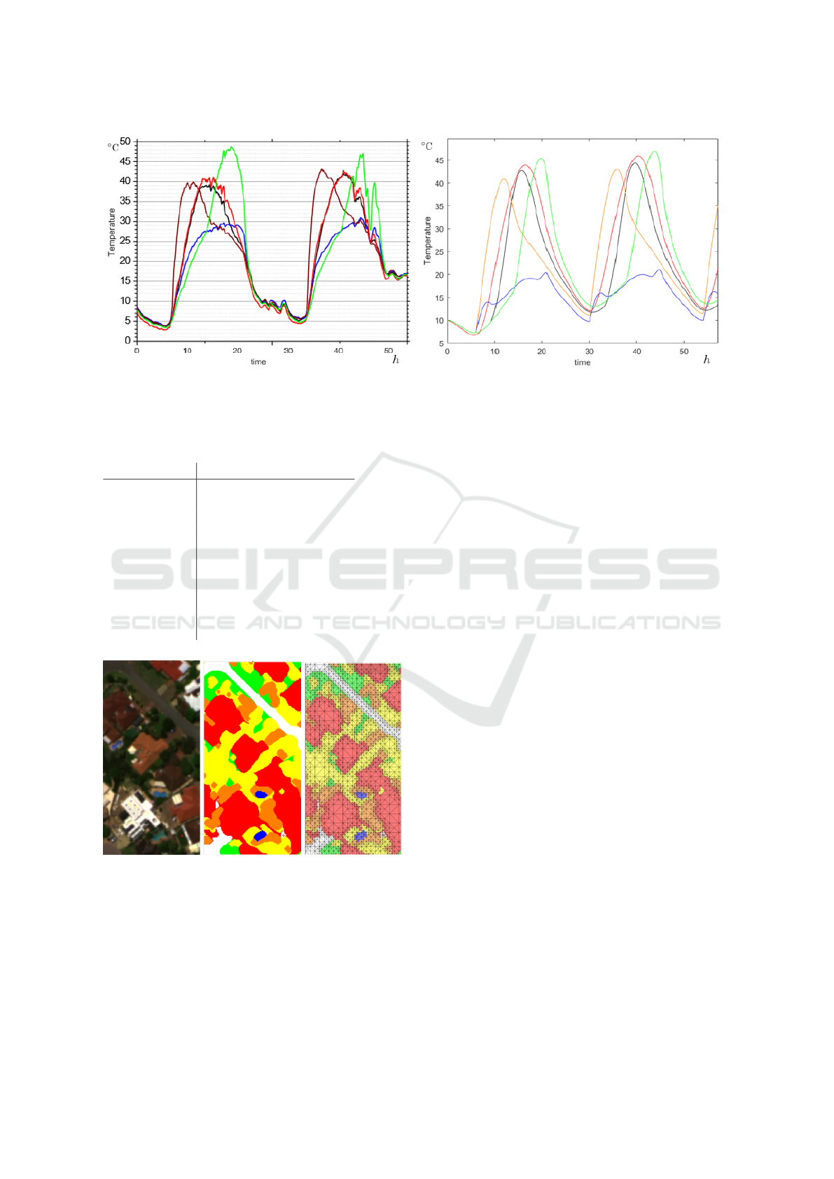
(a) Measured data (b) Simulated data

Figure 8: Measured and simulated temperatures for May 11 and 12, 2006, for thermistors 1 (black), 2 (blue), 3 (yellow), 4

(red) and 5 (green).

Table 2: Material classes of Melville data set.

Semantic Class color

Ground cover Street white

Soil orange

Grass green

Brick red

Tree yellow

Water blue

3D Object Building wall

Roof

Forest box wall

Forest box roof

(a) RGB-Image (b) Classiﬁcation

(see Table 2)

Figure 9: Generation of terrain mesh.

tion result of the ground.

In the simulation presented in the following, we

have chosen the forced convection to be neglected

by setting the wind velocity to zero, i.e. regard-

ing a windless scene. As further weather condi-

tions, we used the same as for the CUBI scenario.

The whole scene consists of 1313410 triangles, and

706405 points and 10 sets of material parameters. The

simulation terminated in 252 sec. for ﬁve day-night

cycles.

Figure 10 (a) shows our simulation result, i.e. the

resulting surface temperatures of the city of Melville

at the time 7h00 on a day in September. The struc-

ture of the city is clearly visible and the different ther-

mal behaviour of the materials appears realistic: the

streets are visible as warm areas and the areas with

vegetation are cooler. Figure 11 shows the surface

temperatures of the scene at noon in a slanted view,

so that the 3D structure becomes visible. Here, the

effect of thermal shadows is demonstrated. They are

visible on surfaces which are not illuminated by the

sun and therefore are exposed to less heating, i.e. the

surface temperature is cooler.

The thermal image of the city of Melville results

from several measurements during night time and al-

lows a ﬁrst comparison between our simulation result

and actual sensor data. Figures 10(b) shows a smaller

region of our simulation result at nighttime and Fig-

ure 10(c) the corresponding thermal image. In direct

comparison, our heat simulation shows good agree-

ment with the thermal image. We have successfully

reproduced the strong signature of the streets during

night and the cooling effect by trees on the streets,

which can punctually be seen along the long road on

the left side of both images. Merging several trees

and modeling them as forest boxes proves to be con-

venient, e.g. the surrounding tree areas around the

large grass ﬁeld return a reasonable surface temper-

ature. Differences between simulation and the ther-

mal image appear considering effects by shadow cast.

GRAPP 2019 - 14th International Conference on Computer Graphics Theory and Applications

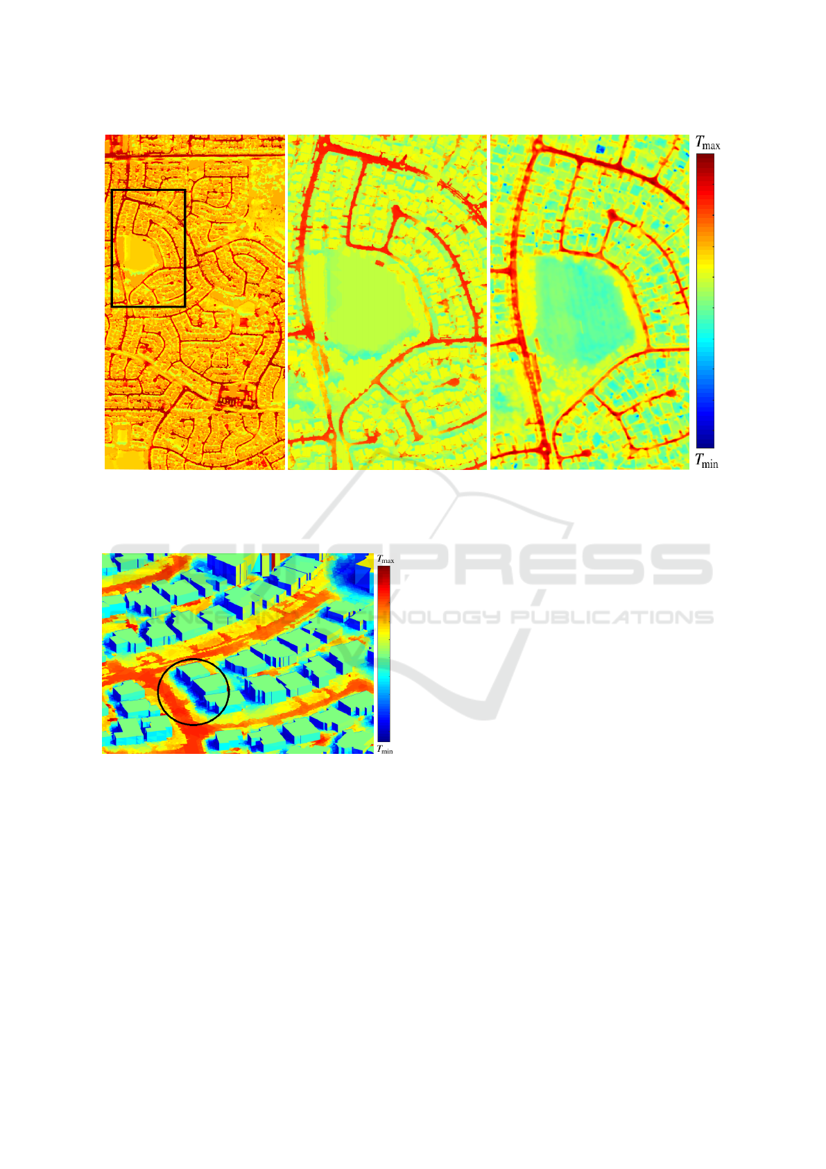
(a) Simulation result (topview) for

the city of Melville at 7h00

(b) Simulated Surface Temperatures (c) Thermal Infrared Image

Figure 10: Comparison between simulated temperatures and thermal infrared image.

Figure 11: Slanting view on the simulation results for the

city of Melville at noon. Areas not directly exposed to sun-

light heat up less and generate thermal shadows (circle).

Within the simulation, shadow casts lead to strong

cooling which is not present in the thermal sensor im-

age. Furthermore, building roofs show a considerably

lower temperature then in the simulation. We suspect

that this is due to the material properties, in particular

a low emissivity, which makes objects appear cooler

on thermal images than they actually are. Field mea-

surements might give more information about the ac-

tual rooﬁng temperatures to enable an evaluation of

these differences.

5 CONCLUSIONS

In this paper, we have presented a thermal simula-

tion approach for large scenes in the framework of

a pipeline leading from raw sensor data to 3D en-

vironments rendered in the infrared spectrum. The

preceding work of the thermal simulation consists of

the material classiﬁcation and mesh generation from

the sensor data. Given the triangulation, we deﬁne a

surface volume as simulation element for discretiza-

tion of the heat transfer equation. Our model results

in qualitatively good agreement between simulation

and ground truth data for small geometries such as

the CUBI object. Applied to a large data set using

the entire pipeline up to thermal simulation, we have

shown that our method efﬁciently leads to similar sur-

face temperatures as compared to a thermal image.

Outstanding signatures in the thermal image are rec-

ognizable in the simulation at a comparable point in

time. Furthermore, the simulation with time displays

the dependency of the solar irradiation and the result-

ing thermal shadows as we expected. Completing the

pipeline towards infrared rendering, where the heat

radiance is modeled, will lead to an optimized start-

ing point for comparison between thermal imaging

and simulation. Also, modeling the heat radiation in

future work will be a promising tool for urban heat

island consideration and other applications.

Physically-based Thermal Simulation of Large Scenes for Infrared Imaging

ACKNOWLEDGEMENTS

We express our deep gratitude to the City of Melville

and Dr. Petra Helmholz from Curtin University, Aus-

tralia, for the acquisition of the Melville data set as

well as Rebecca Ilehag from Karlsruhe Institute of

Technology, Germany, for data preparation. We thank

our colleagues Jonas Mispelhorn for providing the

OpenGL renderer and Dr. Jochen Meidow for read-

ing parts of the manuscript.

REFERENCES

Bartos, B. and Stein, K. (2015). FTOM-2D: a two-

dimensional approach to model the detailed thermal

behavior of nonplanar surfaces. In Target and Back-

ground Signatures, volume 9653, page 96530G. Inter-

national Society for Optics and Photonics.

Biljecki, F., Ledoux, H., and Stoter, J. (2016). An improved

LoD speciﬁcation for 3D building models. Comput-

ers, Environment and Urban Systems, 59:25–37.

Breiman, L. (2001). Random forests. Machine learning,

45(1):5–32.

Bulatov, D., H

aufel, G., Meidow, J., Pohl, M., Solbrig, P.,

and Wernerus, P. (2014). Context-based automatic

reconstruction and texturing of 3D urban terrain for

quick-response tasks. ISPRS Journal of Photogram-

metry and Remote Sensing, 93:157–170.

Council of City of Meville (2017). Urban forest strategic

plan 2017-2036: Plan a: City-controlled plan. Tech-

nical report, City of Melville, Perth, Australia.

Decaudin, P. and Neyret, F. (2004). Rendering forest scenes

in real-time. In EGSR04: 15th Eurographics Sympo-

sium on Rendering, pages 93–102. Eurographics As-

sociation.

Dewan, A. M. and Corner, R. J. (2014). Impact of land use

and land cover changes on urban land surface temper-

ature. In Dhaka Megacity, pages 219–238. Springer.

Feng, X. and Myint, S. W. (2016). Exploring the effect of

neighboring land cover pattern on land surface tem-

perature of central building objects. Building and En-

vironment, 95:346–354.

Gross, H. and Th

onnessen, U. (2006). Extraction of lines

from laser point clouds. International Archives of

Photogrammetry, Remote Sensing and Spatial Infor-

mation Sciences, 36 (Part 3/W49):86–91.

aufel, G., Bulatov, D., and Solbrig, P. (2017). Sensor data

fusion for textured reconstruction and virtual repre-

sentation of alpine scenes. In Earth Resources and

Environmental Remote Sensing/GIS Applications VIII,

volume 10428, page 1042805. International Society

for Optics and Photonics.

Ilehag, R., Bulatov, D., Helmholz, P., and Belton, D. (2018).

Classiﬁcation and representation of commonly used

rooﬁng material using multisensorial aerial data. In-

ternational Archives of the Photogrammetry, Remote

Sensing & Spatial Information Sciences, 42(1).

Johnson, K., Curran, A., Less, D., Levanen, D., Marttila,

E., Gonda, T., and Jones, J. (1998). MuSES: A new

heat and signature management design tool for virtual

prototyping. In Proc. of the 9th Annual Ground Target

Modelling and Validation Conference.

Kajiya, J. T. (1986). The Rendering Equation. In Proc.

of the 13th Annual Conference on Computer Graphics

and Interactive Techniques, SIGGRAPH ’86.

Lagouarde, J.-P., H

enon, A., Kurz, B., Moreau, P., Irvine,

M., Voogt, J., and Mestayer, P. (2010). Modelling

daytime thermal infrared directional anisotropy over

toulouse city centre. Remote Sensing of Environment,

114(1):87–105.

Lienhard IV, J. H. and Lienhard V, J. H. (2011). A heat

transfer textbook. Dover Publ., Mineola, NY, 4. ed.,

corr., rev. and updated edition.

Malaplate, A., Grossmann, P., and Schwenger, F. (2007).

Cubi: a test body for thermal object model validation.

In Infrared Imaging Systems: Design, Analysis, Mod-

eling, and Testing XVIII, volume 6543, page 654305.

International Society for Optics and Photonics.

Mar

echal, N., Gu

erin, E., Galin, E., M

erillou, S., and

erillou, N. (2010). Heat transfer simulation for mod-

eling realistic winter sceneries. In Computer Graphics

Forum, volume 29, pages 449–458. Wiley Online Li-

brary.

Pajarola, R. (2002). Overview of quadtree-based terrain tri-

angulation and visualization. Technical report, De-

partment of Information & Computer Science, Uni-

versity of California, Irvine.

Poglio, T., Savaria, E., and Wald, L. (2002). Outdoor scene

synthesis in the infrared range for remote sensing ap-

plications. In CISST’02: International Conference on

Imaging Science, Systems, and Technology. CSREA

Press, Athens, Ga, USA.

Siegel, R. and Howell, J. R. (1992). Thermal radiation heat

transfer. Francis & Taylor, Washington, DC, 3. ed.

edition.

Sonntag, D. (1990). Import new values of the physical con-

stants of 1986, vapour pressure formulations based on

the ITS-90, and psychrometer formulae. Z. Meterol,

70:340.

Xiong, B., Elberink, S. O., and Vosselman, G. (2014).

Building modeling from noisy photogrammetric point

clouds. ISPRS Annals of the Photogrammetry, Remote

Sensing and Spatial Information Sciences, 2(3):197–

204.

Xiong, X., Zhou, F., Bai, X., Xue, B., and Sun, C. (2016).

Semi-automated infrared simulation on real urban

scenes based on multi-view images. Optics Express,

24(11):11345–11375.

GRAPP 2019 - 14th International Conference on Computer Graphics Theory and Applications