Surgical Phase Recognition of Short Video Shots based on Temporal

Modeling of Deep Features

Constantinos Loukas

Medical Physics Lab, Medical School, National and Kapodistrian University of Athens,

Mikras Asias 75 str., Athens, Greece

Keywords: Surgery, Video, Classification, CNN, LSTM, Deep Learning.

Abstract: Recognizing the phases of a laparoscopic surgery (LS) operation form its video constitutes a fundamental

step for efficient content representation, indexing and retrieval in surgical video databases. In the literature,

most techniques focus on phase segmentation of the entire LS video using hand-crafted visual features,

instrument usage signals, and recently convolutional neural networks (CNNs). In this paper we address the

problem of phase recognition of short video shots (10s) of the operation, without utilizing information about

the preceding/forthcoming video frames, their phase labels or the instruments used. We investigate four

state-of-the-art CNN architectures (Alexnet, VGG19, GoogleNet, and ResNet101), for feature extraction via

transfer learning. Visual saliency was employed for selecting the most informative region of the image as

input to the CNN. Video shot representation was based on two temporal pooling mechanisms. Most

importantly, we investigate the role of ‘elapsed time’ (from the beginning of the operation), and we show

that inclusion of this feature can increase performance dramatically (69% vs. 75% mean accuracy). Finally,

a long short-term memory (LSTM) network was trained for video shot classification, based on the fusion of

CNN features and ‘elapsed time’, increasing the accuracy to 86%. Our results highlight the prominent role

of visual saliency, long-range temporal recursion and ‘elapsed time’ (a feature ignored so far), for surgical

phase recognition.

1 INTRODUCTION

Laparoscopic surgery (LS), a common type of

minimally invasive surgery (MIS), provides not only

substantial therapeutic benefits for the patient, but

also the opportunity to record the video of the

operation for reasons such as documentation,

technique evaluation, skills assessment, and

cognitive training of junior surgeons (Loukas et al.

2011),(Lahanas et al. 2011). However, a major

technological challenge is the effective content

management of the recorded videos, given that an

operation may last for more than an hour, whereas

the duration of yearly operations per surgeon may

exceed 1000 hours (Petscharnig and Schöffmann

2018).

The traditional way of classifying/retrieving

videos relevant to a particular feature of the

operation is via text mining from manual

annotations. Apart from the operation type, the

annotation may include keywords such as a special

technique performed, anatomic characteristics, or

instruments utilized. However, this type of labelling

has some limitations, preventing the effective

management, representation and indexing of the

recorded videos. First, manual annotation is tedious

and time-consuming. Second, semantic

characteristics that are discovered to be of the

surgeon’s interest at a later stage, are excluded from

future searches. Third, global annotation of terms

provides limited information about their time-stamp,

unless this is manually inserted. In most cases, the

surgeon performs manual skimming of the video to

locate the object/event of interest, which is

inefficient. In order to provide surgeons with

additional tools for video content management, an

effective way for video content representation is

essential.

Automated surgical phase recognition from the

LS video is an important topic of research, usually

defined as ‘surgical workflow analysis’ (SWA). The

phases of a surgical operation constitute its

fundamental temporal units, where the surgeon

attempts to complete an overall task before

Loukas, C.

Surgical Phase Recognition of Short Video Shots based on Temporal Modeling of Deep Features.

DOI: 10.5220/0007352000210029

In Proceedings of the 12th International Joint Conference on Biomedical Engineering Systems and Technologies (BIOSTEC 2019), pages 21-29

ISBN: 978-989-758-353-7

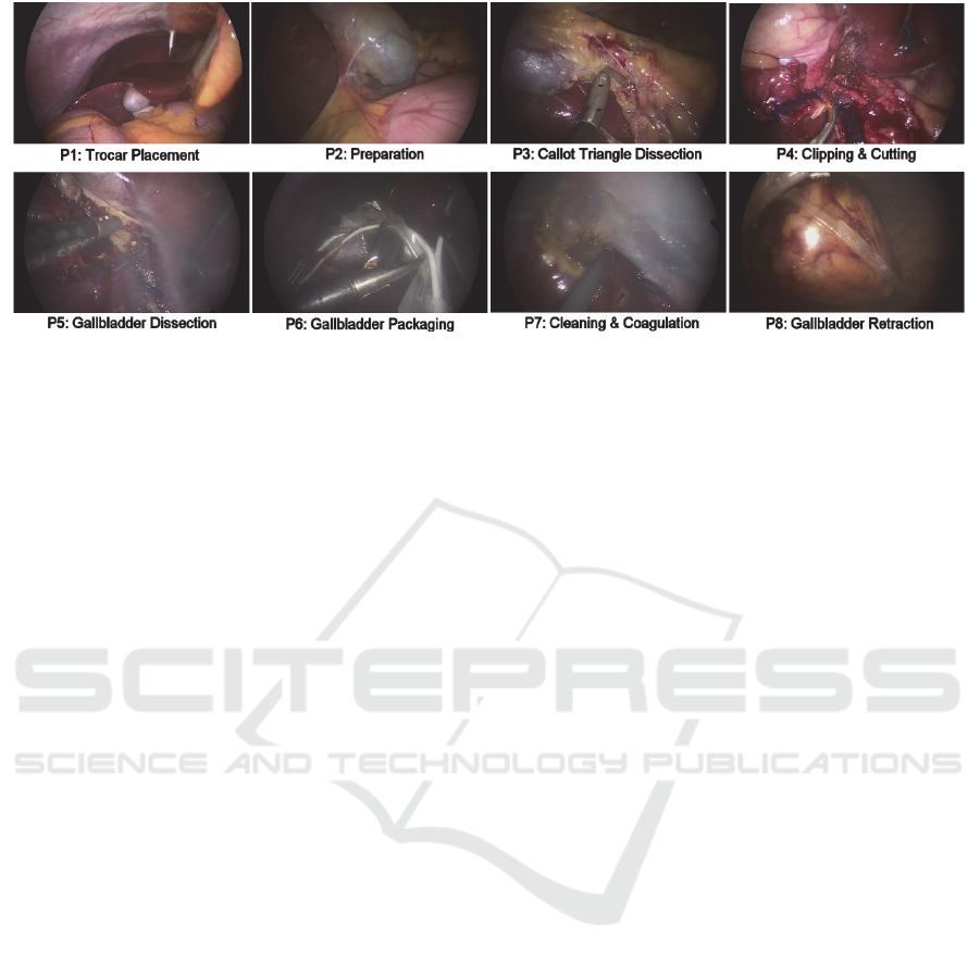
Figure 1: An overview of the 8 surgical phases (P1-P8). The frames were extracted from the annotations of a single LC

operation.

advancing to the next phase. During the phase, the

surgeon manipulates certain anatomic tissues with

the surgical instruments, some of which may be

specific to its label. Surgical phases are of crucial

importance for the structure of the operation as they

correspond to the top hierarchy level according to

the ‘operation decomposition’ model: phases, steps,

tasks/events, and gestures, as described in a recent

review (Loukas 2018). Hence, a method able to

recognize the phase of a surgical operation would

offer solutions to various challenges encountered in

surgical video content management systems. Other

applications include phase-based skills assessment,

automatic selection of didactic content, and

improved OR scheduling (if phase recognition is

performed online).

Initial SWA works employed tool usage signals

from RFID and electromagnetic (EM) sensors as

well as manual annotations, based on the hypothesis

that a surgical phase is characterized by a certain

hand gesture or/and tool usage pattern (Loukas and

Georgiou 2013),(Bouarfa et al. 2011),(Padoy et al.

2012). However, employment of additional sensors

may interfere with the operational workflow and

there are concerns whether these data can be

automatically acquired in the operating room.

Visual features extracted from the recorded video

of the operation seem a more straightforward option

due to the endoscopic camera employed. Compared

to endoscopic examinations, surgical videos present

significant challenges such as presence of smoke

(coagulation), heavy interaction with the operated

organs (dissection/clipping/cutting), and frequent

camera motion as well as tool insertion/removal.

Prior works on vision-based phase recognition

included hand-engineered features based on color,

texture, intensity gradients, or combinations of them

(Lalys et al. 2012). In (Blum et al. 2010), gradient

magnitudes, histograms and color values were

employed. After dimensionality reduction based on

tool usage signal data, laparoscopic cholecystectomy

(LC) operations were segmented into 14 phases with

accuracy close to 77%. The combination of visual

features with tool usage signals was also employed

in (Dergachyova et al. 2016). In another study,

phase border detection of LC videos was performed

via image-based instrument recognition (Primus et

al. 2016).

The aforementioned works employ handcrafted

features, which are specifically designed to capture

certain type of information ignoring other image

characteristics. Recently, deep learning approaches

(e.g. Convolutional Neural networks-CNNs) have

shown promising results for phase recognition. For

example, Twinanda et al. proposed the EndoNet

architecture, a CNN based on the AlexNet

architecture, which was fine-tuned on a dataset of 40

LC operations for the task of tool and phase

recognition (Twinanda et al. 2017). The precision of

offline and online phase recognition was close to

85% and 74% respectively. In the recent M2CAI

2016 challenge for online phase recognition of LC

operations, Jin et al. achieved a mean jaccard score

of 78.2% (the challenge allowed a 10s margin in the

predictions). Their method combined feature vectors

extracted from a fine-tuned ResNet50 CNN

architecture combined with a long-short term

memory (LSTM) network to encode temporal

information (Jin et al. 2018). These works focus on

the online segmentation of the entire operation based

on fully supervised training and using visual

information from the preceding video frames as well

as their inferred phase labels. Recently, a CNN-

based method for video shot classification of

laparoscopic gynecologic actions was proposed in

(Petscharnig and Schöffmann 2017). Video shots of

BIOIMAGING 2019 - 6th International Conference on Bioimaging

the entire course of each surgical action were

employed for training and testing.

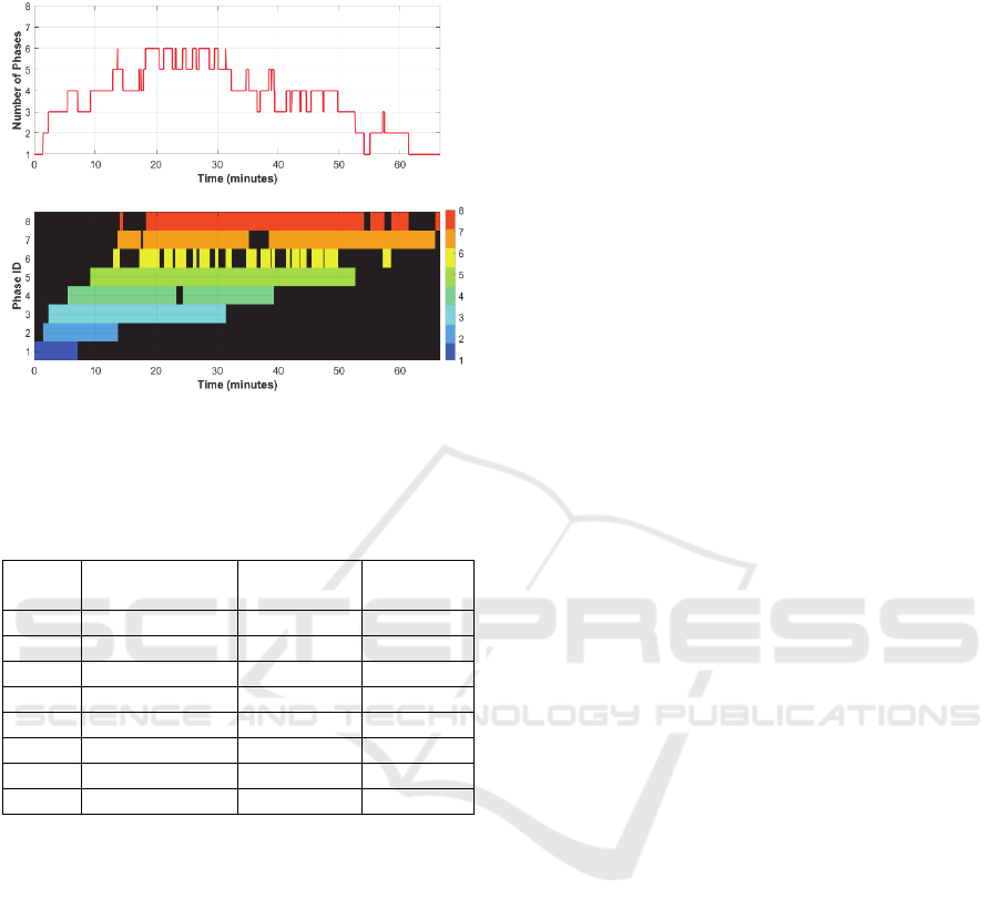
Figure 2: Graphical overview of the number of

simultaneously occurring phases (top) and the temporal

span of each phase (bottom), across the dataset of 27

surgical operations.

Table 1: Statistical overview of the phases.

Phase

mean ± std

(minutes)

min

(minutes)

max

(minutes)

P1 3.04 ± 1.70 1.42 7.08

P2 1.71 ± 2.06 0.35 11.03

P3 10.53 ± 7.97 1.95 26.82

P4 4.70 ± 2.87 0.94 12.39

P5 10.40 ± 6.30 1.68 24.11

P6 1.14 ± 0.59 0.28 3.03

P7 5.68 ± 2.80 1.01 15.97

P8 4.93 ± 5.61 0.66 22.26

In this paper we present a method for phase

recognition from short video shots (10s) of surgical

operations, without any prior knowledge about the

preceding/forthcoming video frames, phase labels or

instruments used. We concentrated on LC which is a

fundamental operation for junior surgeons. Each

video shot essentially represented only a small

fraction of the entire phase. Prompted by the

advances in image classification based on deep

learning approaches, we investigated four state-of-

the-art CNN architectures (Alexnet, VGG19,

GoogleNet, and ResNet101), for feature extraction

via transfer learning. Features were extracted from

two different types of receptive fields: one based on

traditional frame resize to match the CNN’s input

size and another one based on the most salient

region of the input image. Video shot representation

was performed via two temporal pooling

mechanisms. Initially, video shot classification was

based on the 1

nearest-neighbour (NN) using two

different distance metrics. Most importantly, we

investigated the role of absolute ‘elapsed time’ (from

the beginning of the operation), in video shot

classification and we present results that show that

the inclusion of this feature can increase

performance dramatically. Finally, we fused the

CNN features with ‘elapsed time’ and applied long-

range temporal recursion to estimate the probability

of each surgical phase for a video shot, which

improved even further the classification

performance.

2 METHODOLOGY

2.1 Video Shot Dataset

In this work we employed surgical videos from the

M2CAI 2016 Challenge Dataset, which includes

video recordings of complete LC operations

(Twinanda et al. 2017),(Stauder et al. 2016). In

particular, we analyzed 27 video recordings (about

19 hours total duration), from the ‘workflow-train’

sub-dataset. The videos are recorded at 25 frames

per second (25 fps), with full HD resolution

1920×1080. Each video includes frame-by-frame

annotations of the 8 surgical phases of LC: P1)

Trocar Placement, P2) Preparation, P3) Calot

Triangle Dissection, P4) Clipping & Cutting, P5)

Gallbladder Dissection, P6) Gallbladder Packaging,

P7) Cleaning & Coagulation, and P8) Gallbladder

Retraction. Sample frames of the surgical phases are

presented in Figure 1. It may be seen that some

phases may present distinct image characteristics

(e.g. P1, P8), whereas others (e.g. P5-P7) are quite

challenging for visual recognition due to their

similarity or/and presence of smoke (e.g. see P5, P6,

P7).

It should be emphasized that not all operational

phases are sequential and they are governed by some

temporal constraints: P6, P7, P8 are not always

sequential (P6 may occur after P7, or/and P7 after

P8), P7 may occur 2 times, and P7 may not be

present at all. However, phases P1-P5 are always

present in an operation and occur sequentially. A

statistical overview of the phases is presented in

Table 1. It may be seen that P2 and P6 have the

shortest duration whereas P3 and P5 have the

longest one.

Figure 2 shows the number of simultaneously

occurring phases as well as the timings of each

phase, across all 27 video recordings, in the same

diagram. From the top diagram it may be seen that

Surgical Phase Recognition of Short Video Shots based on Temporal Modeling of Deep Features

up to the first 10 minutes, about 1-3 phases may

occur (from P1-P4), and the same is valid after the

50th min (from P5-P8). From the bottom diagram it

may be seen that the order of the phases is relatively

fixed and their duration is limited (e.g. P1-P5).

Furthermore, some phases present almost no

temporal overlap (e.g. P1 vs. P4-P8 and P2 vs. P6-

P8), whereas some others present moderate overlap

(e.g. P1 vs. P3 and P2 vs. P5). From this analysis it

is evident that the absolute temporal position of a

video frame (with regard to the beginning of the

operation), is a crucial factor that should be

considered in phase recognition.

Based on the aforementioned dataset, we

extracted the video shot dataset which was employed

for classification. In particular, for each video and

for each of the 8 phases, we extracted 2 non-

overlapping shots of 10s duration (i.e. 250 frames).

The video shots were extracted from random

temporal positions of each phase, ensuring that the

first/last frame of each shot was within the temporal

limits of each phase. In two videos, P7 was absent so

in order to have an equal number of shots per phase,

we randomly selected 50 (out of 54) shots for each

of the P1-P6 and P8 phases, leading to a total

number of 400 video shots, equally distributed

across the 8 phases.

2.2 CNN Feature Extraction

Feature extraction was based on transfer learning

using ‘off-the-shelf’ features extracted from four

state-of-the-art CNNs: Alexnet, VGG19, GoogleNet,

and Resnet101. These network architectures were

chosen as they are known to perform well on

surgical endoscopy images (Petscharnig and

Schöffmann 2018). Transfer learning implies that

the CNNs were pretrained, in this case on the

Imagenet database which contains millions of

natural images distributed in 1000 classes. Although

surgical images are substantially different, given the

powerful architecture of the CNNs and the huge

volume of Imagenet, transfer learning has been

proved a simple, yet good-working approach for

content-based description of surgical images

(Petscharnig and Schöffmann 2017). Moreover, our

dataset is considerably small to train these CNNs

from scratch. However, as will be discussed later,

we perform training to model the temporal variation

of the extracted CNN features.

Alexnet consists of eight layers: 5 convolutional

layers followed by 3 fully-connected (FC) layers.

For each frame in a video shot, we extracted features

from layer fc7, which is the before-final-fc (BFFC)

layer with length n1=4096. VGG19 is much deeper,

consisting of 16 convolutional layers followed by 3

fully connected layers. We again extracted features

from the BFFC layer (fc7, n2=4096). GoogleNet is

different to Alexnet and VGG19, including various

Inception modules with dimensionality reduction

and only one fully connected layer combined with a

softmax layer (22 layers in total). For each frame we

used the features extracted from the BFFC layer:

pool5-7x7_s1 (n3=1024). Finally, the Resnet101

model is the deepest of the four (101 layers); it

stacks several residual blocks in-between the

convolutional blocks aiming to alleviate the

vanishing gradient problem, usually encountered

when stacking several convolutional layers together.

For the ResNet101 model we used the bottleneck

features extracted from the BFFC layer: pool5

(n4=2048).

Based on the aforementioned approach we

extracted feature descriptors from each video frame.

In order to achieve a compact feature representation

of the video shot, we concatenate the descriptors

along the temporal dimension and apply two

temporal pooling mechanisms: max-pooling and

average-pooling. The former extracts the maximum

value from each dimension of the BFFC layer,

whereas the second one outputs the average from

each dimension of the BFFC layer. For each CNN

architecture employed, both approaches result in a

single feature descriptor for each shot, equal to the

size of the corresponding BFFC layer.

2.3 CNN Input and Saliency Maps

The size of the input layer of the aforementioned

CNNs is: 227×227 (Alexnet) and 224×224 (VGG19,

GoogleNet, and ResNet101). In previous works, the

original image is resized either to match the CNN’s

input, or so that the smaller side matches one side of

the CNN input layer and then the center crop is used

as input to the CNN (Petscharnig and Schöffmann

2017),(Varytimidis et al. 2016). However, both

approaches have some limitations. Considering that

the original video resolution is 16/9, the former case

leads to a spatial degradation of the original image,

as the aspect ratio is forced to be 1 (see Figure 3). In

the latter case, image resizing does not affect the

aspect ratio, but extracting features from the center

crop may lead to an efficient representation of the

original frame since the structures of interest are not

always in the center (w.r.t. Figure 1, in P1 the trocar

is located towards the upper-right corner whereas in

P4 the clips/tool-tip are in the bottom).

BIOIMAGING 2019 - 6th International Conference on Bioimaging

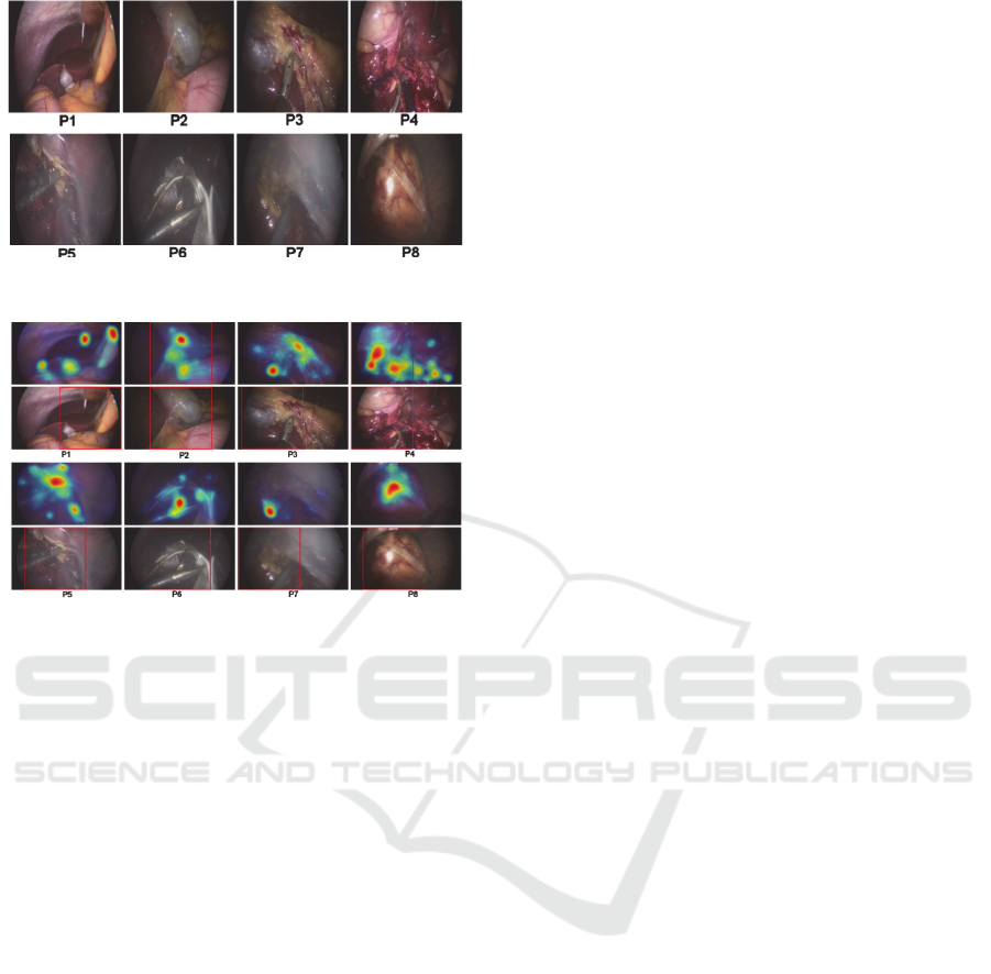
Figure 3: The images shown in Fig. 1, resized to 224×224.

Figure 4: The saliency maps overlaid on the images shown

in Fig. 1 (top) and the rectangular patches which were

used as input to the CNN (bottom).

In this work, we propose an alternative

mechanism for region selection based on visual

saliency. Integration of visual saliency in CNN-

based content-based image representation is a major

trend nowadays. The main idea is to generate a

saliency map that represents the most salient regions

of the input image, without any prior assumption,

based on various criteria such as color- and texture-

contrast (Leboran et al. 2017),(Cheng et al. 2015).

Recent works have shown that using as input to the

CNN a salient, instead of a center/resized crop,

image provides better classification results (Obeso et

al. 2017). In this work we have employed the static

version of the adaptive whitening saliency (AWS)

methodology, which has shown superior

performance in predicting human attention (Leboran

et al. 2017). Recently, this method was applied for

keyframe extraction from video shots of LC

operations (Loukas et al. 2018). In brief, the model

employs a bank of 2D LogGabor filters, generating a

series of filter response maps, which are then

accumulated to generate the final saliency map of

the image.

For the purpose of this work, first we resized the

original full HD frame of the video shot so that the

smaller side (height) matched one side of the CNN

input layer (i.e. 224 or 227). Second, we computed

the saliency map of the resized frame based on the

AWS model. Third, we computed the 5 strongest

local maxima of the saliency map using a

neighborhood size 9×9. Fourth, the spatial

coordinates of these maxima were averaged

providing the center location of an image patch that

was used as input to the CNN. In case the center

location was so that the patch lied outside the resized

frame, the patch was shifted to lie within the frame

window. Finally, a feature descriptor was extracted

from the BFFC layer of the CNN, as described

previously.

Figure 4 provides the saliency maps overlaid on

the corresponding resized frames shown in Figure 1.

Below are the rectangular patches (in this case

224×224), which were used as input to the CNN. It

may be seen that most of the structures of interest lie

within the image patch, such as the trocar in P1, the

gallbladder in P2, the tools in P3-P7, and the

retrieval bag in P8.

2.4 Video Shot Classification based on

Temporal Pooling

Video shot classification was based on the 1st NN

using two different distance metrics: Euclidean and

cosine. For both metrics we used the compact

feature representation of each shot based on the

max- and average-pooling mechanisms, described

before. The Euclidean metric simply takes the L2

norm of the compact feature descriptors whereas the

cosine distance is defined as one minus the cosine of

the included angle between the descriptors. Each of

the 400 compact feature descriptors of the

corresponding video shots was treated as a candidate

descriptor, for which the class is predicted based on

its nearest distance among all other descriptors

(treated as training descriptors). The results were

obtained separately for each combination of pooling

mechanism and distance metric.

As described in Section 2.1, the time-stamp of

the video frames seem to play an important role in

the prediction of the surgical phase. Hence, we also

investigated the effect of adding the time-stamp of

the video shot as an additional dimension to the

CNN features (n+1). Consequently, each video shot

was represented by the pooled CNN descriptor

concatenated by the time stamp of the shot (taken as

the elapsed time, T

elapsed

, of the 1

frame of the shot

from the beginning of the operation).

Surgical Phase Recognition of Short Video Shots based on Temporal Modeling of Deep Features

2.5 Video Shot Classification based on

Temporal Modeling

A significant limitation of the aforementioned

pooling mechanisms for the video shot

representation, is that the resulting descriptor does

not take into account the temporal order of the

individual frames. In other words, if one shuffles the

frames of a video shot, then each of these

mechanisms will lead to the same feature descriptor.

However, the order of the frames (and so the

extracted CNN descriptors) is an important piece of

information that should be utilized in the

classification task. A recurrent neural network

(RNN) exhibits dynamic temporal behaviour for a

time sequence, as the connections between nodes

form a directed graph along the sequence. Moreover,

RNNs use their internal state to process input

sequences and they are able to connect previous

information to the present task, such as using

previous video frames for the understanding of the

present frame and eventually the class of the entire

video shot.

In this work, the CNN feature extraction process

was applied at each time point of the shot, leading to

a temporal order of feature descriptors. Then, we

employed the LSTM network, a special kind of

RNNs, composed of a series LSTM units (as many

as the number of shot’s descriptors), and a FC layer

with softmax at the end to perform classification into

the eight phases. To training parameters of the

LSTM network were similar to those proposed

recently in (Li et al. 2018): batch size=16, training

epochs=80, hidden units=200, learning rate=0.001,

the Adam method for optimization and cross-

entropy as loss function.

Similarly to the aforementioned idea of

concatenating the compact CNN shot descriptor with

the time-stamp of the video shot, here we employed

as input to the LSTM network the CNN features

(extracted from each frame of the shot),

concatenated with the time-stamp of the

corresponding video frame (dimensionality: n+1).

The model was run on every 25th frame (i.e. 1 fps)

to reduce the computational cost. During

training/testing the temporal order of the feature

descriptors was preserved. The LSTM network was

trained on 50% of the video shot dataset (i.e. 200

video shots) and the remaining 50% served as the

test set. We performed 5 random cycles of training,

making sure that a video shot was included at least

once in a training cycle, and then we averaged the

evaluation metrics (see next section).

3 EXPERIMENTAL RESULTS

The performance of the aforementioned approaches

was evaluated in terms of the following metrics:

Acc = (TP + TN)/(P + N) (1)

Pre = TP/(TP + FP) (2)

Rec = TP/(TP + FN) (3)

F1 = 2 × Pre × Rec/(Pre + Rec) (4)

where: Acc, Pre, Rec, F1 denote Accuracy,

Precision, Recall, and F1-score, respectively; TP,

TN, FP, FN, P, N denote: true positives, true

negatives, false positives, false negatives, positives

and negatives, respectively.

Table 2 shows average classification results

using CNN features extracted from the resized raw

images, for the two temporal pooling mechanisms

and the two distance metrics. It is worth noting that

for a particular CNN and pooling mechanism, the

distance metrics are similar, except for ResNet101

where Euclidean leads to worse results for average

pooling. With regard to the two pooling

mechanisms, max pooling seems to yield better

performance, especially when used with cosine, for

all CNNs. The best performance was achieved by

Table 2: Classification results based on resized raw images (Features: CNN).

CNN

type

Pooling: Max

Distance: Cosine

Pooling: Average

Distance: Cosine

Pooling: Max

Distance: Euclidean

Pooling: Average

Distance: Euclidean

Acc Pre Rec F1 Acc Pre Rec F1 Acc Pre Rec F1 Acc Pre Rec F1

alex

net

.60 .60 .61 .61 .59 .60 .59 .60 .59 .60 .60 .60 .56 .58 .57 .57

google

net

.60 .61 .62 .61 .55 .55 .56 .55 .60 .60 .61 .61 .53 .53 .54 .53

vgg19 .60 .61 .61 .61 .57 .56 .57 .57 .60 .61 .60 .60 .56 .57 .57 .57

resnet

101

.64 .65 .64 .64

.61 .64 .61 .62

.65 .66 .65 .65

.57 .59 .58 .58

BIOIMAGING 2019 - 6th International Conference on Bioimaging

ResNet101 (~65%) using max-pooling with either

distance metric.

Table 3: Classification results based on salient maps

(Features: CNN).

CNN

type

Pooling: Max, Distance: Cosine

Acc Pre Rec

alexnet

0.62 0.61 0.62 0.61

googlenet

0.63 0.65 0.64 0.64

vgg19

0.61 0.61 0.62 0.62

resnet101

0.69 0.70 0.70 0.70

Pooling: Max, Distance: Euclidean

alexnet

0.57 0.57 0.57 0.57

googlenet

0.60 0.61 0.61 0.61

vgg19

0.60 0.60 0.61 0.60

resnet101

0.68 0.68 0.68 0.68

Table 4: Classification results based on salient maps

(Features: CNN and T

elapsed

CNN

type

Pooling: Max, Distance: Cosine

Acc Pre Rec

alexnet

0.71 0.73 0.71 0.71

googlenet

0.70 0.72 0.70 0.70

vgg19

0.71 0.72 0.71 0.71

resnet101

0.75 0.76 0.75 0.75

Pooling: Max, Distance: Euclidean

alexnet

0.68 0.68 0.68 0.68

googlenet

0.61 0.61 0.61 0.61

vgg19

0.65 0.65 0.66 0.65

resnet101

0.68 0.68 0.68 0.68

Table 5: Classification results based on salient maps and

LSTM (Features: CNN and T

elapsed

CNN

type

Acc Pre Rec

alexnet

0.73 0.74 0.73 0.72

googlenet

0.81 0.82 0.81 0.81

vgg19

0.78 0.77 0.78 0.77

resnet101

0.86 0.88 0.86 0.86

Table 3 summarizes the classification results

using features extracted from the most salient region

of the image, as described in Section 2.3. Average-

pooling is omitted as it was proved to yield worse

results. Compared to Table 2 it is clear that

extracting features from the most salient image patch

leads to 2-5% improvement for both distance metrics

and for all CNNs. The cosine distance produced

better results (by 3-5%), for all CNNs. The best

performance was achieved again by ResNet101

(~70%), whereas the other three CNNs had similar

performance (61-65%) although higher than that

shown in Table 2.

Table 4 presents the results using the CNN

features extracted from the salient patch,

concatenated with the ‘elapsed time’ feature.

Compared to Table 3, there is a notable

improvement by ~5-10% for all metrics, CNN

architectures, and distance metrics (except for

GoogleNet/ResNet101 with Euclidean, which is the

same). Note that the difference in this experiment

was that the feature vector was increased by 1, the

elapsed time of the 1st frame of the shot from the

operation start. Again, the cosine distance produces

better results than Euclidean, for all CNNs (~3-9%

improvement). The best performance was achieved

again by ResNet101, about 5% higher than that

using only the CNN features (75% vs. 70%).

Table 5 provides the results based on LSTM

model training. Similarly to Table 4, the input to the

network was the CNN feature vector extracted from

the most salient region of the video frame,

concatenated with its time-stamp (i.e. elapsed time

from operation start). Clearly the LSTM model

yields superior performance across all metrics,

compared to the naive NN cosine distance with max-

pooling (compare to Table 4). Specifically, the

improvement was about: 2%, 10%, 7% and 11% for

Alexnet, GoogleNet, VGG19, and ResNet101,

respectively. The best performance was achieved

again by ResNet101 (86-88%), whereas the second

best model was GoogleNet (~81%).

Table 6 illustrates the performance of the LSTM

model for the individual classes, using a confusion

matrix. Columns denote the predicted class while

rows indicate the true class. The numbers denote the

prediction percentage with respect to the samples

from a particular class (positives). For phases P1-P4,

the model yields almost perfect predictions, higher

than 94%, and with very low or no confusion among

the other classes. For P7 and P8 the results are also

remarkable: 79% and 87% respectively. The model

seems to slightly confuse P7 with P5 (9%), and

much less with P4 and P8 (~5%). Phase P8 is

slightly confused with P5 and P7 (5% and 8%

respectively). For P5 and P6 the performance is

similar (~72%). P5 is mostly confused with P7

(26%), whereas P6 with P7 (19%) and P4 (10%).

The lower results for P5, P6 may be due to the visual

similarity with P7 as a result of smoke, as depicted

in Figure 1.

Surgical Phase Recognition of Short Video Shots based on Temporal Modeling of Deep Features

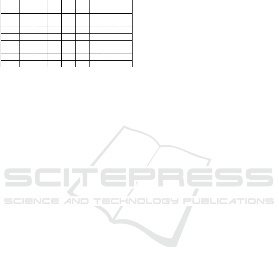
Table 6: Confusion matrix based on salient maps and

LSTM (Features: CNN and T

elapsed

True/

Pred.

P1 P2 P3 P4 P5 P6 P7 P8

.94

.06

P3 .05

.94

.01

.93

.01 .01 .01 .04

.72

.26 .02

P6 .10

.71

.19

P7 .04 .09 .02

.79

.06

P8 .05 .08

.87

4 CONCLUSIONS

In this paper we propose a method for video shot

classification into surgical phases based on deep

features and temporal information modeling. Our

results lead to the following conclusions. First,

extracting CNN features from the most salient

regions of the image allows to achieve better results

(up to 5%). Second, when using a NN approach for

classification, the cosine distance provides better

results (up to 5%). Third, video shot representation

based on max-pooling of CNN image features is

better than average pooling (up to 6%). Fourth,

deeper CNNs provide more robust features for

classification (up to 10% improvement). Fifth,

‘elapsed time’ (a feature ignored so far), can

increase performance dramatically (up to 10% and

6% for shallower and deeper architectures,

respectively). Finally, employing an LSTM model

for temporal modeling of the CNN features fused

with ‘elapsed time’ provides significant performance

improvement: 86% accuracy and 88% precision

(compared to 75% and 76% when max-pooling is

employed, respectively). The investigation of a

visual saliency model specialized to surgical videos,

fine tuning of a ResNet model in which ‘elapsed

time’ is embedded, and other temporal information

modeling architectures, are major topics of interest

for future research work.

ACKNOWLEDGEMENTS

The author thanks Special Account for Research

Grants and National and Kapodistrian University of

Athens for funding to attend the meeting.

REFERENCES

Blum, T. et al., 2010. Modeling and segmentation of

surgical workflow from laparoscopic video. In

Medical Image Computing and Computer-Assisted

Intervention (MICCAI). Lecture Notes in Computer

Science. pp. 400–7.

Bouarfa, L. et al., 2011. Discovery of high-level tasks in

the operating room. Journal of Biomedical

Informatics, 44(3), pp.455–462.

Cheng, M.-M. et al., 2015. Global contrast based salient

region detection. IEEE Transactions on Pattern

Analysis and Machine Intelligence, 37(3), pp.569–582.

Dergachyova, O. et al., 2016. Automatic data-driven real-

time segmentation and recognition of surgical

workflow. International Journal of Computer Assisted

Radiology and Surgery, 11(6), pp.1081–9.

Jin, Y. et al., 2018. SV-RCNet: Workflow recognition

from surgical videos using recurrent convolutional

network. IEEE Transactions on Medical Imaging,

37(5), pp.1114–1126.

Lahanas, V. et al., 2011. Psychomotor skills assessment in

laparoscopic surgery using augmented reality

scenarios. In 17th International Conference on Digital

Signal Processing (DSP). Corfu, Greece: IEEE, pp. 1–

Lalys, F. et al., 2012. A framework for the recognition of

high-level surgical tasks from video images for

cataract surgeries. IEEE Transactions on Biomedical

Engineering, 59(4), pp.966–976.

Leboran, V. et al., 2017. Dynamic whitening saliency.

IEEE Transactions on Pattern Analysis and Machine

Intelligence, 39(5), pp.893–907.

Li, Y. et al., 2018. Context aware decision support in

neurosurgical oncology based on an efficient

classification of endomicroscopic data. International

Journal of Computer Assisted Radiology and Surgery,

13(8), pp.1187–1199.

Loukas, C. et al., 2018. Keyframe extraction from

laparoscopic videos based on visual saliency detection.

Computer Methods and Programs in Biomedicine,

165, pp.13–23.

Loukas, C. et al., 2011. The contribution of simulation

training in enhancing key components of laparoscopic

competence. The American Surgeon, 77(6), pp.708–

715.

Loukas, C., 2018. Video content analysis of surgical

procedures. Surgical Endoscopy, 32(2), pp.553–568.

Loukas, C. and Georgiou, E., 2013. Surgical workflow

analysis with Gaussian mixture multivariate

autoregressive (GMMAR) models: a simulation study.

Computer Aided Surgery, 18(3–4), pp.47–62.

Obeso, A.M. et al., 2017. Connoisseur: classification of

styles of Mexican architectural heritage with deep

learning and visual attention prediction. In 15th

International Workshop on Content-Based Multimedia

Indexing (CBMI). Florence, Italy, pp. 1–7.

Padoy, N. et al., 2012. Statistical modeling and

recognition of surgical workflow. Medical Image

Analysis, 16(3), pp.632–41.

BIOIMAGING 2019 - 6th International Conference on Bioimaging

Petscharnig, S. and Schöffmann, K., 2018. Binary

convolutional neural network features off-the-shelf for

image to video linking in endoscopic multimedia

databases. Multimedia Tools and Applications, pp.1–

26.

Petscharnig, S. and Schöffmann, K., 2017. Learning

laparoscopic video shot classification for

gynecological surgery. Multimedia Tools and

Applications, 77(7), pp.8061–79.

Primus, M.J. et al., 2016. Temporal segmentation of

laparoscopic videos into surgical phases. In 14th

International Workshop on Content-Based Multimedia

Indexing (CBMI). Bucharest, Romania: IEEE, pp. 1–6.

Stauder, R. et al., 2016. The TUM LapChole dataset for

the M2CAI 2016 workflow challenge. ArXiv,

1610.09278.

Twinanda, A.P. et al., 2017. EndoNet: A deep architecture

for recognition tasks on laparoscopic videos. IEEE

Transactions on Medical Imaging, 36(1), pp.86–97.

Varytimidis, C. et al., 2016. Surgical video retrieval using

deep neural networks. In Medical Image Computing

and Computer-Assisted Intervention (MICCAI)-

M2CAI Workshop. Athens, Greece, pp. 4–14.

Surgical Phase Recognition of Short Video Shots based on Temporal Modeling of Deep Features