
Incorporating Plane-Sweep in Convolutional Neural Network Stereo
Imaging for Road Surface Reconstruction
Hauke Brunken and Clemens G
¨
uhmann
Chair of Electronic Measurement and Diagnostic Technology, Technical University of Berlin,
Einsteinufer 17, 10587 Berlin, Germany
Keywords:
Stereo Vision, Neural Network, Plane Sweep, Pavement Distress.
Abstract:
Convolutional neural networks, which estimate depth from stereo pictures in a single step, have become state
of the art recently. The search space for matching pixels is hard coded in these networks and in literature is
chosen to be the disparity space, corresponding to a search in the cameras viewing direction. In the proposed
method, the search space is altered by a plane sweep approach, reducing necessary search steps for depth map
estimation of flat surfaces. The described method is shown to provide high quality depth maps of road surfaces
in the targeted application of pavement distress detection, where the stereo cameras are mounted behind the
windshield of a moving vehicle. It provides a cheap replacement for laser scanning for this purpose.
1 INTRODUCTION
Knowledge about the road surface is useful in several
cases, such as road maintenance, driving assistance
systems and active suspension systems.
At present for the purpose of road maintenance,
specially equipped measuring vehicles are utilized,
which use laser scanners to generate a road profile
(Eisenbach et al., 2017). Alternatively people are
send to observe and measure roads by hand. This is
costly and time consuming. As the road surface can
change quickly, for example when a pothole develops,
the gathered information becomes outdated.
Another subject are driving assistance or autono-
mous driving systems, where potholes should be ci-
rcumvented or the driving speed should be reduced
due to bad road conditions. Active suspension sys-
tems can utilize depth information to provide the best
driving comfort.
This work aims at solving the problem of recon-
structing the road surface ahead of a moving vehicle
by stereo vision. This is a difficult task, as roads have
a low texture surface and surface defects produce little
change in elevation. The developed system could be
mounted on public vehicles, such as public transpor-
tation or garbage trucks in order to provide current
data for many roads with little effort. Changes in road
conditions can be detected early, which can lead to sa-
vings in repair costs. While laser scanners capture the
world serially, cameras can capture the entire image in
parallel. This is advantageous at high driving speeds,
as is the case with driver assistance or autonomous
driving systems.
The proposed method is an extension of neural
networks for disparity estimation by implementing
plane sweep stereo into the network. It is trained end-
to-end on data, which was created by a more traditi-
onal plane sweep approach. The final network learns
from the training data and even outperforms the met-
hod it learned from in some cases.
Results are shown for the targeted application and
are compared to a laser scan.
2 RELATED WORK
Depth estimation from stereo images is a well-known
problem (Hartley and Zisserman, 2003), (Szeliski,
2011), (Ikeuchi, 2014). It can be broken down to ma-
tching pixels in left and right camera images. The
location of a point in 3D space can then be found by
triangulation. The corresponding pixel of a pixel in
one image lies on the epipolar line in the other image.
If the cameras are aligned horizontally, the epipolar
line is located in the same row in the second image as
the pixel in question in the first image. Traditionally
this pixel matching procedure is divided into several
stages:
1. If the cameras are not (perfectly) aligned horizon-
784
Brunken, H. and Gühmann, C.
Incorporating Plane-Sweep in Convolutional Neural Network Stereo Imaging for Road Surface Reconstruction.
DOI: 10.5220/0007352107840791
In Proceedings of the 14th International Joint Conference on Computer Vision, Imaging and Computer Graphics Theory and Applications (VISIGRAPP 2019), pages 784-791
ISBN: 978-989-758-354-4
Copyright
c
2019 by SCITEPRESS – Science and Technology Publications, Lda. All rights reserved

tally, the pictures are rectified.
2. A similarity measure between each pixel in one
image and each pixel on the same horizontal line
in the other image is calculated.
3. The similarity measure is used to match pixels of
both images. Due to ambiguities, wrong matches
can easily occur if only the similarity measure is
taken into account. This makes an additional cost
function and complex optimization necessary.
Different similarity measures have been utilized. A
very efficient one is a convolutional neural network,
which outperforms traditional methods like sum of
absolute differences, census transform and norma-
lized cross-correlation (Zbontar and LeCun, 2016).
This gave rise to the idea of integrating the second
and third steps into a single neural network. Diffe-
rent architectures thereof exist. In (Dosovitskiy et al.,
2015) a network for estimating optical flow is propo-
sed. That means, a field around a pixel in consecu-
tive frames of a video sequence needs to be searched.
If left and right pictures of a stereo camera are used
as input, the flow corresponds to disparity. The idea
thus was modified for stereo images in (Mayer et al.,
2016), where a correlation layer is used to account
for the epipolar geometry. In (Kendall et al., 2017)
the idea of a cost volume is introduced. First, fea-
ture maps for left and right images are calculated in
the network. Then feature maps of different disparity
levels of one image are stacked on top of the feature
maps of the other image. This approach embeds the
epipolar geometry. In (Smolyanskiy et al., 2018) a
similar network with a semi-supervised training pro-
cedure is implemented, which can run near real-time.
Besides Flownet (Dosovitskiy et al., 2015), all
these methods search through disparity space, which
corresponds to a search in the cameras viewing di-
rection. This creates two problems in the targeted ap-
plication:
1. Since the cameras are mounted behind the winds-
hield, the angle between the viewing direction of
the cameras and the road is sharp. For the task of
depth estimation of the surface, many small steps
through disparity space are necessary to get a high
depth resolution of the surface.
2. The other problem is the rectification of images.
To produce a high depth resolution, the baseline
between cameras has to be large. This in turn re-
quires the cameras to be tilted in, in order to get
an overlap of the images in the region of interest.
In this case, rectification can result in a reduction
of quality, due to the required stretching and inter-
polation.
Both problems are solved by the plane sweep appro-
ach, which was first introduced in (Collins, 1996):
A virtual plane is placed at arbitrary positions in 3D
space. Features of both images are projected onto the
plane and match if the plane’s position is correct. In
(Yang et al., 2003) this approach is used to warp entire
images for dense scene reconstruction.
In this work, a neural network is extended by a
plane sweep approach, in which feature maps are war-
ped by a plane homography inside the network. By
projecting the feature map of one camera onto the
plane and into the other camera, rectification becomes
unnecessary, and, more importantly, by sweeping the
virtual plane from below to above the road surface,
the search space is reduced. The network is trained
on a dataset, which was created by a plane sweep ap-
proach in conjunction with semi global matching.
3 METHOD
The method described in this paper consists of an ex-
isting convolutional neural network for disparity esti-
mation, which is modified to estimate change in sur-
face elevation by a plane sweep approach. The plane
sweep direction is perpendicular to the road surface
and therefore a plane must be found which represents
the mean road surface. This plane is guessed initially
and refined later on.
In this section first the idea of plane sweep and
its usage is described. Next, the convolutional neu-
ral network on which this work is based on is briefly
recapitulated. Subsequently the embedding of plane
sweep into this network is described. At the end it is
shown how the mean surface can be found.
3.1 Plane Sweep
The left camera image of a plane, that is parallel to
the x-y-plane, is calculated by the 2D homography
(Collins, 1996)
H
L,i
= K
L
r
L,1
r
L,2
z
i
r
L,3
+ t
L
. (1)
K
L
is the camera matrix. The camera location is given
by the columns of the rotation matrix r
L,{1,2,3}
and the
translation vector t
L
. z
i
is the distance between the x-
y-plane and the parallel plane.
To find the plane parts of a pair of images was ta-
ken of, both images can be back projected onto virtual
planes i by the inverse homographies H
−1
L,i
and H
−1
R,i
,
where H
R,i
is the homography for the right camera. If
the plane is at the correct position for these parts of
the images, they will match on the virtual plane. This
Incorporating Plane-Sweep in Convolutional Neural Network Stereo Imaging for Road Surface Reconstruction
785
Leftimage
Rightimage
siamesenetworks
featuremap
network
3D
network
Depthmap
stack
feature
maps
featuremap
network
interpolation
&
regression
warpbyplane
homographies
H
i
4Dcostvolume
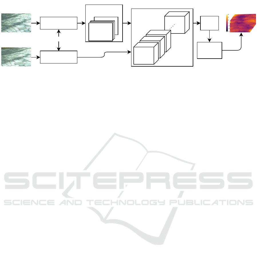
Figure 1: Feature maps are calculated by a Siamese network for both input images. One of them is transformed by a plane
homography and a 4D cost volume is created. Matching is done by the 3D network, which outputs the depth map.
idea was introduced in (Collins, 1996), where sparse
image features are back projected.
In this work dense feature maps are generated by
a neural network. The feature map of the left image is
back projected onto virtual planes and projected into
the right camera, where matching is performed by the
neural network. The back and forth projection is des-
cribed by
H
i
= H
R,i
· H
−1
L,i
. (2)
Performing the matching in the camera space instead
of the plane space has several advantages: Images –
or feature maps in this case – are not stretched much,
which is the case if the virtual plane is not parallel to
the camera. The shape of the cost volume stays the
same, no matter of the perspective the plane induces.
Besides, that way only the feature map of one image
has to be transformed.
3.2 Neural Network for Disparity
Estimation
Different architectures of neural networks for depth
estimation exist, as was laid out in Section 2. The
plane sweep extension can be added to all networks
which are based on the idea of a cost volume. Here
the work of (Chang and Chen, 2018) is incorporated,
as it is able to exploit global context information. By
creating image features with the help of spatial py-
ramid pooling, region-level features instead of pixel-
level features are introduced (Chang and Chen, 2018).
As roads have little texture, it is believed that region-
level features will improve the overall performance,
especially if cracks or other contexts are visible.
Their network consists of four parts: A Siamese
network that creates feature maps from input ima-
ges at a reduced resolution, concatenation of these
feature maps, creating a 4D cost volume, a 3D net-
work, which calculates the cost for each disparity
value for every location, upscaling by interpolation,
and a regression function. The feature map network
gets rectified 3-channel images as input with reso-
lution W × H (with times height) and creates F fe-
ature maps with resolution W /4 × H/4 per image.
The cost volume is assembled according to disparity
space. That means, for each considered disparity va-
lue, the feature maps of the reference image are stac-
ked on top of the shifted feature maps of the other
image. This produces a cost volume of dimension
W /4 × H/4 × D/4 x 2F. D is the number of consi-
dered disparity values. The 3D network converts the
4D cost volume into a 3D cost volume of dimension
W /4 × H/4 × D/4 by 3D convolutions, which is up-
scaled by trilinear interpolation to the original resolu-
tion of W × H × D. Now a regression function finds
the best fitting disparity value by regressing over the
D values at every location. The regression function is
ˆ
d =
D
max
∑
d=0
d · σ(−c
d
), (3)
where σ() is the softmax operation, d are the disparity
values, D
max
is the maximum disparity and c
d
is the
cost value.
3.3 Neural Network for Surface Depth
Map Estimation
In the proposed method the assembly of the cost vo-
lume is altered according to plane sweep. First P pla-
nes parallel to the road surface are proposed. The
right image is taken as reference, thus the left fea-
ture maps need to be warped by the induced homo-
graphies. For every proposed plane, the feature maps
of the reference image are stacked on top of the war-
ped feature map of the other image. This produces a
cost volume of dimension W/4 x H/4 x P x 2F. The
3D network and regression function are left unchan-
ged. The upscaling function changes, as that it does
not have to upscale the disparity (plane, respectively)
dimension. An overview of the method is shown in
Figure 1.
VISAPP 2019 - 14th International Conference on Computer Vision Theory and Applications
786

Warping of the feature maps is accomplished by
inverse warping (Szeliski, 2011): Coordinates of
every pixel of the reference image are transformed by
the inverse of the plane induced homography (Equa-
tion 2). The result is a lookup table. The feature
maps of the left image are copied with the help of
this lookup table, which is first rounded to the nearest
integer coordinate. As the neural network generates
features maps at a lower resolution compared to the
input images, the camera matrices have to be scaled
before applying Equation 2.
One might be tempted to use a more sophisticated
approach as in spatial transformer networks (Jader-
berg et al., 2015), where bilinear interpolation is used.
In our experiments this does not work. The neural
network has a large receptive field (Chang and Chen,
2018), which, in conjunction with interpolation, pre-
sumably breaks the relation between an image pixel
and its corresponding value in the feature map. Du-
ring evaluation bilinear interpolation can be utilized.
Training is performed end-to-end on depth maps,
with the target being the index of the virtual planes.
The usage of the index is similar to the usage of dis-
parity in Section 3.2. That way, the network is inde-
pendent of the actual depth values and different plane
hypothesis can be proposed while training and evalu-
ating.
3.4 Locating the Mean Road Surface
As the plane sweep is conducted from below to above
the mean surface, its location has to be known in ad-
vance. An initial plane can be guessed, as the approx-
imate positions of the cameras in relation to the road
are known. The location is then refined: A depth map
is created by the neural network and is then back pro-
jected to 3D space, resulting in a 3D point cloud in
the camera coordinate system. A grid of points is ex-
tracted as a subset to save some calculation time. A
plane, which best resembles the point cloud, is then
found by a random sample consensus (RANSAC) al-
gorithm (Fischler and Bolles, 1981). In that the mean
of the point cloud is subtracted. Singular value de-
composition is utilized, which directly gives the rota-
tion matrix from the camera coordinate system to the
plane coordinate system, in which the x-y-plane re-
sembles the mean surface. It is located in the center of
the road. The subtracted mean is the translation vec-
tor. To find the final r
{L/R},{1,2,3}
and t
{L/R}
, which
are used in Equation 1, the transformation between
camera centers and camera coordinate system has to
be accounted for.
To generate a bird’s-eye view later, it is useful
to place the camera coordinate system in the center
between the cameras. The rotation between camera
coordinate system and plane can then be composed
by a rotation around the x-axis, followed by a rotation
around the y-axis. Thus, the rotation matrix is disas-
sembled to Euler angles, the rotation around the z-axis
is set to 0 and the rotation matrix is reassembled. This
ensures that the birds-eye-view does not get rotated if
it is shown in the road coordinate system.
After locating the mean surface, the neural net-
work is evaluated a second time.
4 EXPERIMENTS
In the following section the system setup, the training
procedure and the evaluation is described.
4.1 System Setup
Two Basler acA1920-150uc global shutter color ca-
meras with 25 mm lenses are employed. The sen-
sors have an optical size of 2/3” with a resolution of
1920×1200 pixels. The pixel size is 4.8µm × 4.8 µm.
The cameras are mounted on a rig behind the winds-
hield of a vehicle. As the distance between cameras
and road is large (up to 13 m at the upper edge in Fi-
gure 2) and the depth resolution needs to be high (ele-
vation differences of a road are in the mm scale), the
baseline has to be as large as possible. Due to the flat
geometry, a large baseline does not produce occlusi-
ons. The baseline is set to 1.08 m and camera height
above ground is 1.4 m. In order to have a large over-
lapping part in both pictures, cameras are tilted in by
6
◦
each. The angle between the camera rig and the
road is 13
◦
, in order to look across the hood. This
makes it possible to record an area of approximately
2m × 7m.
The aperture has a big influence on the depth of
field. For the depth of field to be large, it has to
be small. On the other hand the aperture influences
the required shutter time and thereby the motion blur,
thus it has to be large. Even at slow driving speeds the
motion blur predominates. For this reason, the aper-
ture is set to the smallest value of f/1.4 for images
taken while driving and to f/8.0 for standstill images.
As the windshield has an influence on calibration
parameters (Hanel et al., 2016), calibration is perfor-
med with the cameras in their final position.
4.2 Training
The proposed convolutional neural network (refer-
red to as CNN in the following) is pretrained on the
KITTI 2015 dataset. Therefore, the cost volume in
Incorporating Plane-Sweep in Convolutional Neural Network Stereo Imaging for Road Surface Reconstruction
787
(a) (b) (c)
(d) (e) (f)
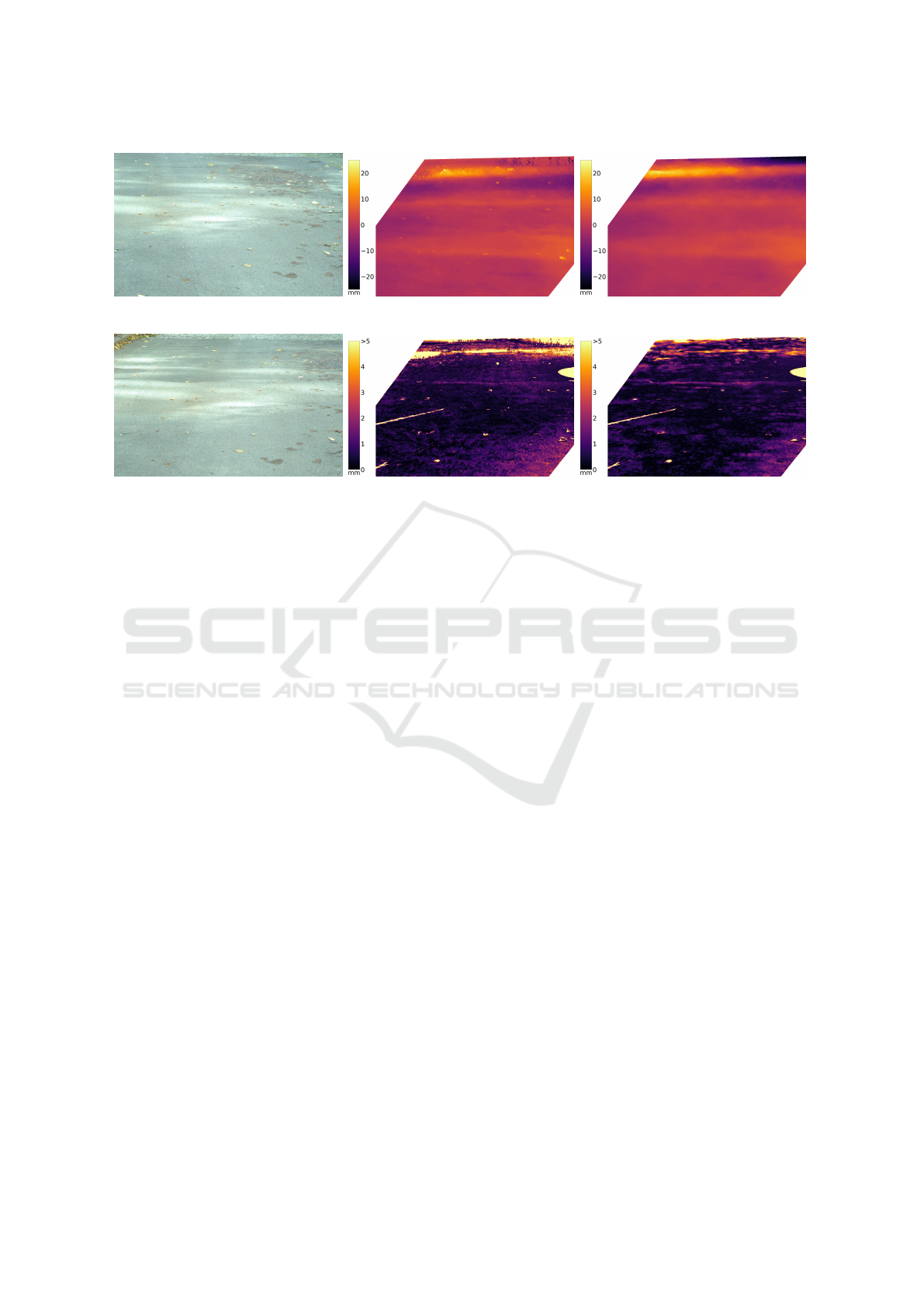
Figure 2: Static scene: a,d left and right image b,c depth map generated by SGM and CNN method (viewed from the right
camera perspective) e,f error between laser scan reference and SGM/CNN method. The circular part on the right and the
stripe on the left are artefacts of the laser scan. The distance between camera and the lower part of the image is 4.5m, between
camera and upper part 13.0m.
the network is assembled as described in Section 3.2.
Learned weights are saved and cost volume assembly
is switched to the plane sweep approach (Section 3.3).
Training is continued with data of the targeted appli-
cation. For the training set depth was extracted by a
stereo method, which is based on a plane sweep ap-
proach in conjunction with semi-global matching (the
method is referred to as SGM) and is out of scope of
this paper. It is based on the work in (Hirschm
¨
uller,
2008). The location of the mean road surface is an
output of the earlier method and is also used for trai-
ning. The training dataset consists of 510 stereo ima-
ges, which were taken while driving. Another 20 still
stereo images were taken outside the vehicle.
Laser scans are not used for training because a suf-
ficiently large data set was not available and is diffi-
cult to obtain. Laser scanning and capture of stereo
images would have to take place simultaneously and
the relationship between scanner and camera would
have to be precisely known. This makes the measu-
rement complex and expensive equipment would be
necessary, especially for the measurements while dri-
ving. Thus, a stereo method is used.
The number of feature maps F is set to 32 and the
number of planes P to 64. Plane sweep is performed
from −30mm to +30 mm around the mean road sur-
face. An example of a training set composed of left
and right color images as input and a depth map as
output can be seen in Figure 2a, 2d and 2b (although
this particular example was used for validation only).
Training is performed on two NVidia GTX 1080
Ti graphics cards (both have 11 GB of memory) in
parallel mode. The model does not fit into memory
in training mode if images with the full resolution of
1920 × 1200 pixels are employed. Thus, 256 × 256
pixel patches of the right image are randomly cho-
sen. The corresponding patch in the left image can be
calculated, as the planes which will be gone through
while sweeping are known in advance. The left image
patch is padded to 576 × 300 pixels in order to have
a uniform size for the learning batch. The principal
points in the camera matrices have to be adjusted ac-
cording to the patch locations. Batch size is set to 8.
In evaluation mode, when no gradients are required
and if intermediate results are deleted, the network
for full resolution images fits into GPU memory of a
single card.
4.3 Evaluation
In order to interpret the results, first the depth resolu-
tion of the camera system is investigated. The method
is then evaluated by a comparison against a laser scan
with standstill images. Afterwards, results from the
targeted application of pavement destress detection
while driving are shown.
VISAPP 2019 - 14th International Conference on Computer Vision Theory and Applications
788
(a)
(b) (c)
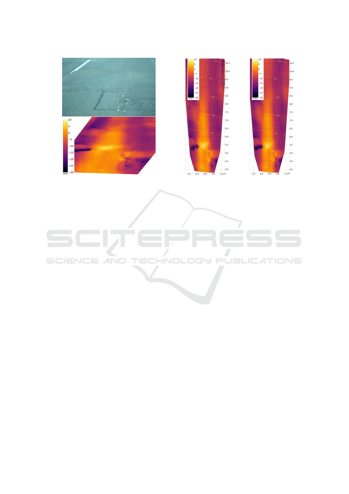
Figure 3: (a) Right image, captured from behind the windshield of a moving car at 37km h
−1
and corresponding depth map
created with CNN method, (b) depth map from a bird’s-eye view with contour lines, indicating depth resolution in mm/pixel
created by SGM method and (c) created by CNN method.
4.3.1 Depth Resolution
For the aforementioned setup, the depth resolution is
calculated as follows: If the correct plane is known
for a pixel in the right camera image, the matching
pixel in the left camera image can be calculated by
the plane homography. If the plane is raised, the mat-
ching pixel will be shifted. The elevation of the plane
divided by the pixel shift is embraced as the resolu-
tion. It is shown as contour lines in Figures 3b and 3c
and in Figure 4 for the central line between cameras.
The exact resolution depends on the relation between
cameras and the mean surface.
4.3.2 Comparison Against Laser Scan
As a reference a laser scan was conducted. The scan-
ner (Z+F IMAGER 5006h) has a range uncertainty of
0.4mm and an uncertainty in vertical and horizontal
direction of 0.007
◦
. This sums up to a total maximal
uncertainty of 0.8 mm in the direction perpendicular
to the road surface in the area of interest. Due to the
high precision of the laser scanner, it is considered to
be the ground truth.
For comparison, the depth maps are projected to
3D space, where the distance to the point cloud of the
laser scanner can be calculated. This is accomplished
with the help of the software CloudCompare (GPL
software, 2017). Because the relation between ca-
mera and laser scanner coordinate system is unknown,
the compared point cloud is rotated and shifted until
both point clouds line up. Then a piecewise quadra-
tic function is fitted through the reference point cloud
and the shortest distance to the compared point cloud
is calculated.
The result is shown for standstill images from the
right cameras perspective in Figure 2e and 2f for the
SGM and CNN methods. SGM refers to the method
which was used to create the training data and CNN
to the proposed method. Images were taken outside
the vehicle while standing still.
It can be seen that both methods are capable of
reconstructing the road surface with high precision.
The mean absolute error (MAE) is 1.1 mm for SGM
and 0.8 mm for the CNN method. The CNN method
did not just learn from the SGM method, it even out-
performs SGM in this example. SGM fails in parti-
cular regions, which can be seen in the upper left and
upper right corner, where CNN produces the correct
depth according to the error image (Figure 2f) and
SGM does not (Figure 2e). The reason presumably
is that in the CNN method region-level features are
employed (Section 3.2). The SGM method produces
correct results for most pixels, while some are wrong.
The correct pixels fit the model, which is tried to be
learned by the neural network. The wrong pixels ap-
pear as noise. Since the correct pixel outweigh the
wrong pixels, the neural network is able to generalize
the correct and to reject the erroneous training data.
Figure 4 shows the MAE of horizontal lines in
bird’s-eye view (refer to Figure 3c) for Figure 2 and
the physical resolution as described in Section 4.3.1
for the central vertical line. The small MAEs of the
entire point clouds compared to the MAEs of hori-
Incorporating Plane-Sweep in Convolutional Neural Network Stereo Imaging for Road Surface Reconstruction
789
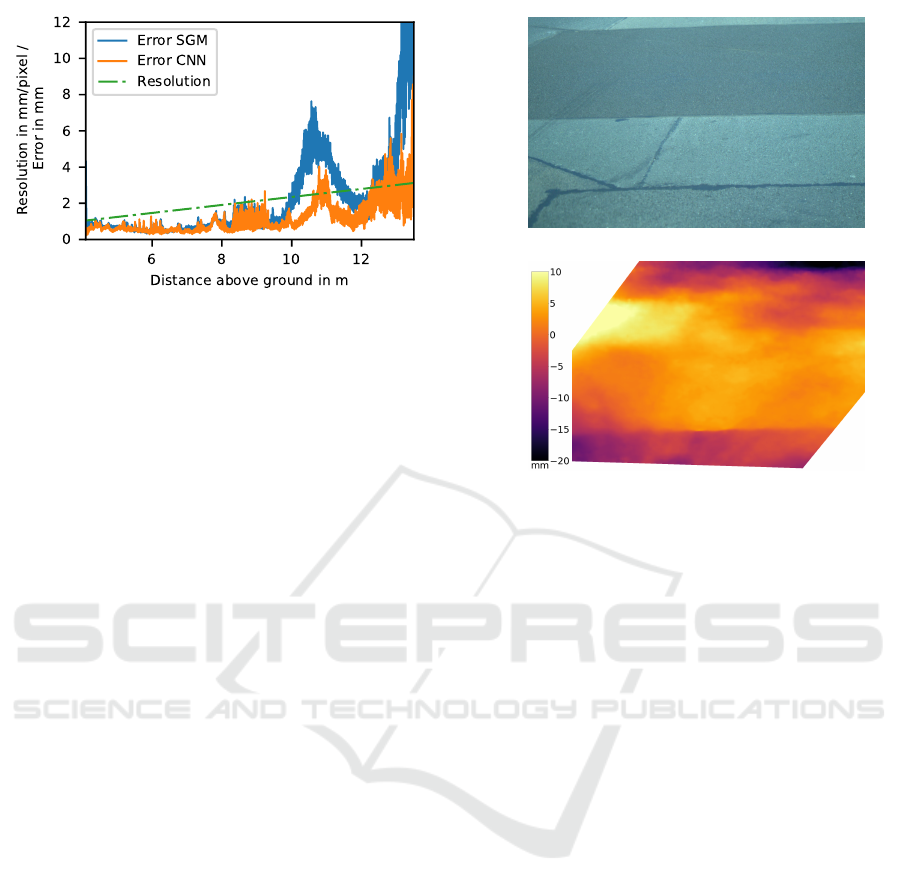
Figure 4: Errors of the SGM and CNN methods compared
to the laser scan are shown, which increase over distance
from the cameras. The physical depth resolution of the ste-
reo camera setup decreases over distance.
zontal lines shown in the graph are caused by the fact
that the density of the point cloud decreases over dis-
tance. Thus, there are more points with small errors
than with large errors. The mean of MAEs of hori-
zontal lines is 2.1 mm for SGM and 1.2mm for CNN.
The sudden increase of the error at 11 m is caused by
the circular artefact of the laser scan (Figure 2e and
2f) and the erroneous section of the SGM method in
the upper left (Figure 2e).
Compared to the physical resolution the errors are
very small, especially when they are close to the ca-
meras. The methods are capable of achieving sub-
pixel accuracy. The SGM method interpolates bet-
ween pixels by plane sweeping and image warping,
while the CNN method uses the regression function
(Equation 3). Another cause is the alignment of point
clouds (Section 4.3.2), which reduces the error artifi-
cially.
4.3.3 Final Application
Figure 3 shows the right camera image and the cor-
responding depth maps from the cameras perspective
and from a bird’s-eye view. The images were ta-
ken from behind the windshield while driving at
37km h
−1
. A repair patch is visible (covering parts
of the lane mark), which is elevated from the road.
Closer to the camera on the left hand side a depres-
sion can be seen. In the lower right several cracks can
be extinguished. If one looks at the bird’s-eye view,
rutting is visible across the entire distance.
The CNN method (Figure 3c) is more robust than
the SGM method (Figure 3b), which can be seen
by looking at the lower left and upper right corners.
Overall the CNN method produces smoother depth
maps.
Figure 5 shows another example at a higher dri-
(a)
(b)
Figure 5: (a) Right image, captured from behind the winds-
hield of a moving car at 75 kmh
−1
and (b) corresponding
depth map created with the CNN method.
ving speed of 75km h
−1
. Although no laser scans are
available for images which were taken while driving,
the results are qualitatively correct. Please note that
the color scales cover different ranges in Figures 2, 3
and 5.
5 CONCLUSION
It was shown how convolutional neural networks for
disparity estimation can be adapted to predict depth
maps of flat surfaces. Results are compared against a
laser scan and show high accuracy over large distan-
ces. The new method even outperforms the method it
learned from in some cases.
The proposed method proves to be very suita-
ble for the challenging task of road surface recon-
struction. It can be utilized to quickly scan road sur-
faces with little effort at driving speeds.
REFERENCES
Chang, J.-R. and Chen, Y.-S. (2018). Pyramid Stereo Ma-
tching Network. arXiv preprint arXiv:1803.08669,
page 9.
Collins, R. T. (1996). A space-sweep approach to true
multi-image matching. In Computer Vision and Pat-
tern Recognition, 1996. Proceedings CVPR’96, 1996
VISAPP 2019 - 14th International Conference on Computer Vision Theory and Applications
790

IEEE Computer Society Conference on, pages 358–
363. IEEE.
Dosovitskiy, A., Fischer, P., Ilg, E., Hausser, P., Hazirbas,
C., Golkov, V., van der Smagt, P., Cremers, D., and
Brox, T. (2015). Flownet: Learning optical flow with
convolutional networks. In Proceedings of the IEEE
International Conference on Computer Vision, pages
2758–2766.
Eisenbach, M., Stricker, R., Seichter, D., Amende, K., De-
bes, K., Sesselmann, M., Ebersbach, D., Stoeckert, U.,
and Gross, H.-M. (2017). How to get pavement dis-
tress detection ready for deep learning? A systematic
approach. In 2017 International Joint Conference on
Neural Networks (IJCNN), pages 2039–2047, Ancho-
rage, AK, USA. IEEE.
Fischler, M. A. and Bolles, R. C. (1981). Random sample
consensus: a paradigm for model fitting with appli-
cations to image analysis and automated cartography.
Communications of the ACM, 24(6):381–395.
GPL software (2017). Cloudcompare 2.8.
Hanel, A., Hoegner, L., and Stilla, U. (2016). Towards the
Influence of a Car Windschield on Depth Calculation
with a Stereo Camera System. ISPRS - International
Archives of the Photogrammetry, Remote Sensing and
Spatial Information Sciences, XLI-B5:461–468.
Hartley, R. and Zisserman, A. (2003). Multiple view geome-
try in computer vision. Cambridge University Press,
Cambridge, UK; New York.
Hirschm
¨
uller, H. (2008). Stereo Processing by Semiglobal
Matching and Mutual Information. IEEE Transacti-
ons on Pattern Analysis and Machine Intelligence,
30(2):328–341.
Ikeuchi, K., editor (2014). Computer Vision - A Reference
Guide. Springer US, Boston, MA.
Jaderberg, M., Simonyan, K., Zisserman, A., and others
(2015). Spatial transformer networks. In Advances in
neural information processing systems, pages 2017–
2025.
Kendall, A., Martirosyan, H., Dasgupta, S., Henry, P., Ken-
nedy, R., Bachrach, A., and Bry, A. (2017). End-
to-End Learning of Geometry and Context for Deep
Stereo Regression. arXiv:1703.04309 [cs]. arXiv:
1703.04309.
Mayer, N., Ilg, E., Hausser, P., Fischer, P., Cremers, D.,
Dosovitskiy, A., and Brox, T. (2016). A large dataset
to train convolutional networks for disparity, optical
flow, and scene flow estimation. In Proceedings of
the IEEE Conference on Computer Vision and Pattern
Recognition, pages 4040–4048.
Smolyanskiy, N., Kamenev, A., and Birchfield, S. (2018).
On the Importance of Stereo for Accurate Depth Es-
timation: An Efficient Semi-Supervised Deep Neural
Network Approach. CoRR, abs/1803.09719.
Szeliski, R. (2011). Computer Vision. Texts in Computer
Science. Springer London, London.
Yang, R., Welch, G., and Bishop, G. (2003). Real-Time
Consensus-Based Scene Reconstruction Using Com-
modity Graphics Hardware. In Computer Graphics
Forum, volume 22, pages 207–216. Wiley Online Li-
brary.
Zbontar, J. and LeCun, Y. (2016). Stereo matching by
training a convolutional neural network to compare
image patches. Journal of Machine Learning Rese-
arch, 17(1-32):2.
Incorporating Plane-Sweep in Convolutional Neural Network Stereo Imaging for Road Surface Reconstruction
791
