A Comparative Study on Voxel Classification Methods for Atlas based
Segmentation of Brain Structures from 3D MRI Images
Gaetan Galisot
1
, Thierry Brouard
1
, Jean-Yves Ramel
1
and Elodie Chaillou
2
1
LIFAT Tours, Universit
´
e de Tours, 64 avenue Jean Portalis, 37000, Tours, France
2
PRC, INRA, CNRS, IFCE, Universit
´
e de Tours, 37380, Nouzilly, France
Keywords:
3D Image Segmentation, Local Atlas, Voxels Classification.
Abstract:
Automatic or interactive segmentation tools for 3D medical images have been developed to help the clinicians.
Atlas-based methods are one of the most usual techniques to localized anatomical structures. They have shown
to be efficient with various types of medical images and various types of organs. However, a registration step
is needed to perform an atlas-based segmentation which can be very time consuming. Local atlases coupled
with spatial relationships have been proposed to solve this issue. Local atlases are defined on a sub-part of
the image enabling a fast registration step. The positioning of these local atlases on the whole image can be
done automatically with learned spatial relationships or interactively by a user when the automatic positioning
is not well performed. In this article, different classification methods possibly included in local atlases seg-
mentation methods are compared. Human brain and sheep brain MRI images have been used as databases for
the experiments. Depending on the choice of the method, segmentation quality and computation time are very
different. Graph-cut or CNN segmentation methods have shown to be more suitable for interactive segmenta-
tion because of their low computation time. Multi-atlas based methods like local weighted majority voting are
more suitable for automatic process.
1 INTRODUCTION
Manual annotation of anatomical structures in 3D me-
dical images is a laborious task for clinicians and bio-
logists. Manual segmentation is still performed slide
by slide and can be very time consuming. Develop-
ment of tools helping to study the different types of
medical images is important. That is why, a lot of au-
tomatic methods have been proposed to provide seg-
mentation on various type of anatomical structures
and organs.
Atlas-based segmentation methods are ones of the
most usual types of techniques used for medical ima-
ges (Cabezas et al., 2011). A training database, com-
posed of several 3D medical images and the labeled
maps associated, is used to build an atlas of an organ.
Then, the segmentation is performed in two steps; the
atlas is first registered to the image that the user wants
to segment, then a segmentation (voxel classification)
method is applied, merging the information coming
from the image and the atlas. Different ways exist to
model a priori information. In particular probabilistic
atlas, multi-atlas or statistical shape model are often
used. In this work, we focus on the volume atlases.
One of the usual drawbacks is the computation
time of the atlas-based methods. The atlas is usually
defined on the whole organ. Then, the segmentation
needs at least one non-linear registration step which is
time consuming when the size or the resolution of the
image is important. We can also note that the atlas-
based segmentation are usually fully automatic and
does not let the opportunity to the user to drive the
segmentation process.
In order to obtain more interactive and faster par-
tial segmentations, local atlases have been proposed
in (Galisot et al., 2017). These atlases are built on a
small part of the image corresponding to the bounding
box of each region. Each anatomical structure is des-
cribed by its own template. Because of the small size
of the sub-image, the registration step is performed in
a faster way. To do the registration, local atlases must
be positioned (superposed) inside the whole image to
be segmented according to the known spatial relati-
onships between regions that have to be learned from
the training dataset. The user has also the possibility
to help the system by re-positioning the borders of
the bounding box of the local atlas inside the whole
image if necessary. By this interaction, the system
Galisot, G., Brouard, T., Ramel, J. and Chaillou, E.
A Comparative Study on Voxel Classification Methods for Atlas based Segmentation of Brain Structures from 3D MRI Images.
DOI: 10.5220/0007358503410350
In Proceedings of the 14th International Joint Conference on Computer Vision, Imaging and Computer Graphics Theory and Applications (VISIGRAPP 2019), pages 341-350
ISBN: 978-989-758-354-4
Copyright
c
 2019 by SCITEPRESS – Science and Technology Publications, Lda. All rights reserved
341

can be driven or optimized by the user if the segmen-
tation result is not satisfactory. The local approach
provides significant advantages compared to the glo-
bal one. First the information about the variability
of the shape is separated from the information about
the positioning positioning. Of course the computa-
tion time for a local registration significantly reduced
compared to a global registration. But, the local seg-
mentation brings also questions about the impact of
the local positioning and registration on the result pro-
vided by voxel classification step. It is important to
study how the different possible voxel classification
methods usually used in global atlas-based approach
are able to deal with a local, incremental and inte-
ractive segmentation way.
Section 2 reminds how the local atlases and spa-
tial relationships are built and used during a segmen-
tation. Section 3 presents six methods of voxels clas-
sification are studied in this paper; hidden Markov
random field, simple voting method, local weighted
voting method, joint label fusion method, Graph-cut
and CNN. In section 4, two databases of brain images
are presented and experiments comparing the diffe-
rent methods are described. Results are discussed in
Section 5, explaining which classification method is
the most suitable based on the experiment results.
2 LOCAL ATLAS
SEGMENTATION
An atlas is an a priori information which needs a clas-
sification method to provide a final segmentation. A
various type of classifications have been described in
literature using either probabilistic or multi-atlas in-
formation. Multi-atlas based segmentation has provi-
ded great results on the segmentation of brain images
(Iglesias and Sabuncu, 2015). A part or the totality
of the training images are registered to the image to
be segment. Voxels classification for multi-atlas have
been mainly based on majority voting method (Rohlf-
ing et al., 2004; Klein et al., 2005) and the most fre-
quent label provided by the training labeled maps is
chosen. Probabilistic atlases encode the probability
to observe an anatomical structure in a certain po-
sition (Shattuck et al., 2008; Nitzsche et al., 2015).
The training images of a population are merged by
registering all the training images to the same space.
They have been combined with a Gaussian mixture
model (Ashburner and Friston, 2005), hidden Markov
random field (Scherrer et al., 2009) or graph-cut met-
hods (Dangi et al., 2017).
The work described in (Galisot et al., 2017), pro-
poses to use different atlases defined locally to loca-
lize anatomical structures. Each anatomical structure
is described by its own atlas. Within this method, du-
ring the learning step, the local atlases and the spatial
relationships between them should be learned from a
database. Thereafter, this learned model can be used
to incrementally segment several anatomical structu-
res in new images. The two following sections ex-
plain the construction of the model.
2.1 Local Atlas
A training database, composed of N couples of MRI
and labeled images, is needed to construct the local at-
lases. Each region is learned independently from each
other. Figure 1 describes the process of construction
of the local atlases.
For each region r, the bounding boxes are detected
in the labeled images and the volume inside is extrac-
ted and denoted by L
r
. The corresponding volume in
the MRI images is also extracted and denoted by B
r
.
In practice, a margin is added around the bounding
boxes. This margin helps to decrease the influence of
a wrong positioning and reduce abrupt frontiers in the
probability maps. In the following, the bounding box
term will refer to this extended bounding box.
At the end of this step, a local multi-atlas is alre-
ady built. Each region r is described by N couples
{B
a
r
,L
a
r
} of images with a = {1,...,N}. Two other
steps are applied if a local probabilistic atlas is requi-
red. An intensity normalization is applied between
the N MRI sub-images B
r
. Then, the local probabilis-
tic atlas for each structure is built incrementally. The
couples {B
a
r
,L
a
r
} of images are registered and the re-
sult is averaged providing a template T
r
and probabi-
lity map Pr
r
.
2.2 Spatial Relationships
As we previously mention, the bounding boxes con-
taining the local atlases can be positioned automati-
cally by the system. Spatial relationships are learned
between regions. These relationships allow to posi-
tion each region compared to the others. In practice,
the regions which are already located will provide in-
formation about the positioning of the next region to
segment. Since these relations depends on the regions
already located, the first region to segment can not be
positioned automatically. The aim is also to, either
help the user by proposing a position and limit the
quantity of his interaction or perform an almost (only
the initialization) fully automatic segmentation.
This spatial information is modeled as distances
between the borders of each region. Relations are
computed independently along the 3 common directi-
VISAPP 2019 - 14th International Conference on Computer Vision Theory and Applications
342

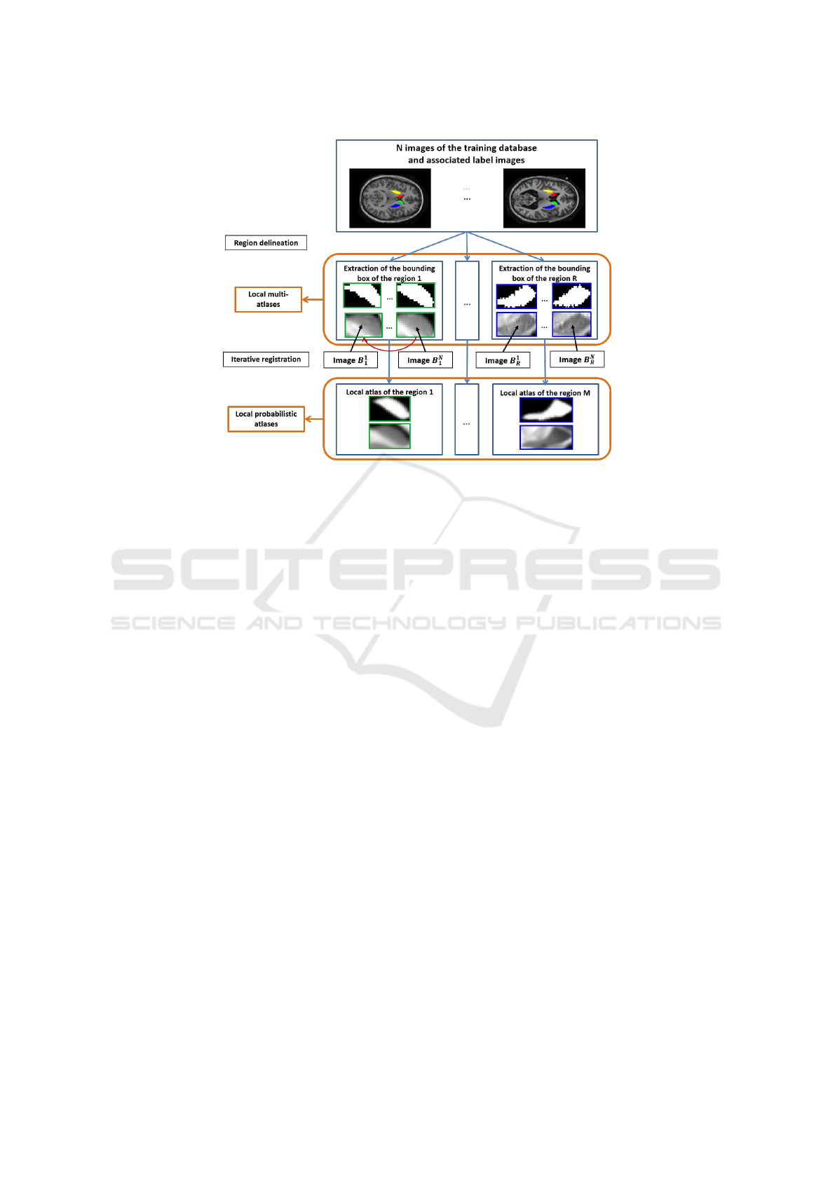
Figure 1: Process of construction of local atlases. Example with two anatomical structures (caudate nucleus, putamen) in
human brain images (Galisot et al., 2017).
ons. In 3D, twelve distances are defined between
two regions. In order to let the system independent
from size or image resolution, distances are normali-
zed compared to the size of the source region. Finally
the minimum and the maximum of relative distances
present in the training database is computed and sto-
red.
During the segmentation, all the regions which are
already segmented will provide information about the
positioning of the next region r to segment. The posi-
tioning of a border of the bounding box is performed
independently from the others. The different intervals
of relative distances are selected and transformed in
the absolute space of the new image. Then, the infor-
mation coming from the different regions and diffe-
rent intervals are merged to obtain a final estimation
of the position of the local atlas. The final position
provides the volume Y
r
which contains in the boun-
ding box.
2.3 Incremental Segmentation
The segmentation using local atlases is performed in-
crementally and in an interactive way. The anatomi-
cal structures are localized sequentially. Contrary to
a classical atlas, each region is described in its own
space. Two different registrations are needed when
two different regions are segmented. However, these
registrations are performed very fast because of the
small size of the different local atlases. Each atlas
must be positioned inside the image to segment. This
positioning can be done by the user. He or she must
position the 6 borders of the bounding box of the re-
gion. This positioning can be also performed using
spatial relationships (cf. Section 2.2). The volume
inside the bounding box is denoted by Y
r
. The local
atlas of the region r is registered to Y
r
.
If a probabilistic atlas is used, the transformation
is determined by the registration of the template T
r
to Y
r
and the same transformation is then applied to
the probability map Pr
r
. If a multi-atlas method is
used, N transformations are computed from B
r
to the
sub-image Y
r
and the same transformation are applied
to the labeled map L
r
. Combination of this registe-
red information with the MRI intensities in Y
r
can be
used as input information for the different classifica-
tion processes discussed in the next section. The seg-
mentation of a region is also definitive, meaning that
the segmentation of a new region does not modify the
result obtained for a previous region.
3 CLASSIFICATION METHOD
After the registration of the local atlas of the volume
Y
r
, a transformation τ is applied on the local proba-
bilistic atlas {B
r
,Pr
r
} (respectively a transformation
τ
a
on the local multi-atlas {B
a
r
,L
a
r
}). In the following,
we will denoted by {B
r
,Pr
r
} and {B
a
r
,L
a
r
} instead of
{B
r
(τ),Pr
r
(τ)} and {B
a
r
(τ
a
),L
a
r
(τ
a
)} respectively. A
voxel classification must be used to obtain the final
segmentation. The process is applied only inside the
A Comparative Study on Voxel Classification Methods for Atlas based Segmentation of Brain Structures from 3D MRI Images
343

sub-volume Y
r
and not on the whole image.
A binary classification can be applied because
only one region is sought in each sub-volume. A large
amount of classification methods have been already
coupled with atlas in the classical case. The follo-
wing section describes these different segmentation
methods we applied for the local approach case. In
the following, Z
r
denotes the binary segmentation of
Y
r
we want to segment.
3.1 Hidden Markov Random Field
Hidden Markov random fields (HMF) are often used
as classifiier with atlas-based methods. It can incor-
porate easily the information coming from the pro-
babilistic atlas as well as the intensities coming from
the MRI images. The images are modeled by an un-
directed graph where the nodes represent the voxels
and the edges represent the adjacency between these
voxels. The HMF used in this works is similar to the
one described in (Scherrer et al., 2009). Y
r
and Z
r
are
considered as random variable field. We denoted z
r
and y
r
, a realization of this random variable. A poste-
riori probability can be expressed in Gibbs form :
p(z
r
|y
r
,φ) = W
−1
exp(−H(z
r
|y
r
,φ)) (1)
With φ the model parameters and H a local energy
which can be then express as follows:
H(z
r
|y
r
,φ) = −
∑
i∈B
r
[α(v)u(v) + β
∑
q∈N (v
0
)
z
r
(v
0
).z
r
(v)
+ log(p(y
r
(v)|z
r
(v),φ))]
The information coming from the atlas for the
voxel v is weighted with the parameter α(v). The
neighborhood information is weighted with the pa-
rameter β. p(y
r
(v)|z
r
(v),φ) denoted the probability
to obtain an intensity if the voxel belong to the re-
gion z
r
(v). Intensities of each class are modeled by a
Gaussian distribution. An initialization is needed and
performed with a K-means algorithm with K classes.
Only one of these classes is selected to be a region
class and driven by the atlas (u(v) = −log(Pr
r
(v))).
The other classes are driven by the exterior of the at-
las (u(v) = −log(1 − Pr
r
(v))).
Segmentation is the obtained by finding the Gaus-
sian parameters maximizing the likelihood. This
maximization is performed with an Expectation-
Maximization algorithm.
3.2 Graph-Cut
In (Boykov et al., 2001), medical images have been
processed with a Graph-Cut (GC) method by taking
into account a user interaction. GC technics have
also been combined and driven by probabilistic atlas
(Dangi et al., 2017) or multi-atlas information (Pla-
tero et al., 2014).
GC segmentation is also based on a Markov field
where the image is described by a graph similarly to
HMF. Moreover, two terminal nodes are added repre-
senting two classes. A source node describing the
region and a sink node describing the background
which are linked to all the other nodes (pixel nodes).
GC segmentation is based on finding the segmenta-
tion minimizing the energy defined as follows :
E(Z
r
) = R (Z
r
) + B(Z
r
) (2)
R (Z
r
) is a region properties term, B(Z
r
) is a
boundary properties term and models a surface pena-
lization. R (Z
r
) is computed with the weights present
on the edges between the voxels and the terminal no-
des. B(Z
r
) is computed with the weights present on
the edges between two voxels.
B(Z
r
) =
∑
p,q∈N
B
p,q
.δ(Z
r
(p),Z
r
(q)) (3)
With δ(l
1
,l
2
) equal to 1 if l
1
is different to l
2
, 0
otherwise. It is commonly depending on the gradient
intensities. The weight between a voxel p and a voxel
q is fixed to B
p,q
=
exp((Y
r
(p)−Y
r
(q))
2
)
2σ
2
. σ is the standard
deviation of the sub-images B
r
.
R (Z
r
) =
∑
v∈Y
r
R
v
(Z
r
(v)) (4)
The regional term can model an a priori informa-
tion about the intensities or the shape but also model
an information coming from the user. In this work,
the regional term brings the probabilistic atlas infor-
mation. R
v
is equal to −log(Pr
r
(v)) for the region
class and equal to log(1 − Pr
r
(v)) for the background
class. The max-flow min-cut algorithm is performed
with the Boykov-Kolmogorov algorithms (boost li-
brary) proposed in (Boykov and Kolmogorov, 2004).
3.3 Majority Voting
Majority Voting is one of the easiest and most com-
mon way to perform the label fusion step of a multi-
atlas segmentation method (Rohlfing et al., 2004;
Klein et al., 2005).
Simple Voting Method. After the registration of
the available local atlases, the labeled L
r
is transfor-
med to the target image space Y
r
. The label of each
voxel in the sub-image Y
r
is then obtained by selecting
the label the most frequently provided by the different
VISAPP 2019 - 14th International Conference on Computer Vision Theory and Applications
344

label maps. We call this the ”simple voting method
(SV)” if no weights are used during the merging step.
The segmentation of the r is defined as follows :
Z
r
(v) = argmax
l={reg/bg}
N
∑
a=1
δ(L
a
r
(v),l) (5)
With δ(l
1
,l
2
) equal to 1 if l
1
is equal to l
2
, 0 otherwise.
Local Weighted Voting Method. Global (Xa-
bier Artaechevarria, 2008) or local weights (Isgum
et al., 2009; Iglesias and Karssemeijer, 2009) have
also proposed to merge information coming from the
labeled maps. The weights are based on the difference
between the registered atlas B
r
and the sub-image Y
r
.
In this works, local weights are applied. The segmen-
tation of the region r is computed as follows :
Z
r
(v) = argmax
l=reg/bg
N
∑
a=1
w
a
(v)δ(L
a
r
(v),l) (6)
Where w
a
(v) is the weight associated to the voxel
v in the atlas a. w
a
(v) is inversely proportional to
the sum square difference between a patch 3 × 3 × 3
around v on Y
r
and B
r
. In the following, this method
is denoted weighted voting method (WV).
3.4 Joint Label Fusion
The Joint Label Fusion method is described in (Wang
et al., 2013). It is also a multi-atlas segmentation met-
hod with the use of local weights. However these
weights are not only based on the similarity between
Y
r
and the atlases, but take into account the correlation
between the atlases. If different atlases seem to bring
similar information, the weights are fixed in such way
that they act like only one atlas. In practice, the weig-
hts are computed in order to minimize the expected
label difference between atlases. A correlation ma-
trix M
v
(a,b) is computed describing the probability
that an atlas a and an atlas b provide the same labe-
ling error at a voxel v. An estimation of this matrix
is proposed by comparing the different atlases and the
target image to segment. The correlation is computed
as follows :
M
v
(a,b) = [h|B
a
r
(N (v)) −Y
r
(N (v))|,
|B
b
r
(N (v)) −Y
r
(N (v))|i]
where N (v) is a neighborhood around the voxel v.
Minimization of the expected label difference leads
to define local weights as :
w
v
=
M
−1
v
1
n
1
t
n
M
−1
v
1
n
(7)
with 1
n
a unitary vector of size n and w
n
a vector of
local weights of a voxel v. The final segmentation is
achieved in the same manner that the local weighted
voting method.
3.5 Convolutional Neural Network
Convolutional Neuron Network (CNN) segmentation
have been also applied on medical images especially
U-net network. First in 2D (Ronneberger et al., 2015),
then in 3D (C¸ ic¸ek et al., 2016), U-net networks per-
form an end-to-end segmentation. CNN process is
not an atlas-based method as the ones described pre-
viously but the network can be train with the same
training database than the one used to built the diffe-
rent atlases.
The different couples of training sub-images
{B
r
,L
r
} have been used to train several networks.
Each of them is built to provide a binary classifica-
tion for one specific anatomical structure. For each
region, the N different couples {B
r
,L
r
} are resized to
a multiple of dimension two. A data augmentation is
performed by applying a random linear transforma-
tion (Random translation, rotation, shear and zoom)
to the sub-images. The network is composed of 3 con-
volutional and 3 deconvolutional layers. Pooling step
are performed between each layers. 100 epochs have
been used to train each CNN.
Similarly to all the previous methods with local
atlases, the sub-image Y
r
is extracted and process by
the CNN of the region r.
4 COMPARATIVE STUDY
4.1 Experiments
Two experiments have been conducted to compare the
different classical methods coupled with the local at-
lases:
• First experiment (E
1
): the different local atlases
are positioned inside the test images according to
the ground truth. The learned spatial relationships
are not used. This situation represent the ideal
case where the user position well each bounding
box.
• Second experiment (E
2
): the efficiency of the dif-
ferent segmentation methods to use the spatial re-
lationships is evaluated. Only the X first regions
are positioned with the ground truth. The other
bounding boxes are positioned automatically ac-
cording to the learned spatial relationships. The
A Comparative Study on Voxel Classification Methods for Atlas based Segmentation of Brain Structures from 3D MRI Images
345

segmentation method have to manage the situa-
tion when the local atlases are not perfectly posi-
tioned inside the whole image.
In the two experiments, the order of segmentation has
been fixed. The specification of the machine used
to execute the experiments is: Intel(R) Xeon(R), E5,
2.20GHz, 4 cores, 8 Go Ram.
4.2 Image Data Bases
Two image databases have been used during the ex-
periments.
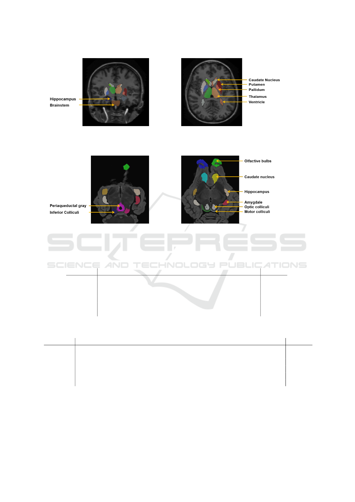
MICCAI. The MICCAI database is a T1 MRI
image dataset of the human brain. This dataset has
been used during a challenge of multi-atlas segmenta-
tion of brain images (Landman et al., 2012). The trai-
ning part is composed of 15 images and testing part is
composed of 20 images. In this work 13 anatomical
structures are used. They represent sub-cortical struc-
tures that are important for disease diagnostic. An ex-
ample of the MICCAI data set is illustrated in Figure
2.
SheepBrain. The SheepBrain is a T2 MRI image
dataset of ex-vivo adult sheep brains. The images
have been acquired by Cyril Poupon (CEA, Neuro-
Spin, Saclay) as part of the NeuroGeo
1
project. Six
brains were acquired with 7T 50 mT/m MRI with a
spatial resolution of 0.3×0.3×0.3 mm. Fifteen ana-
tomical structures have been manually labeled. An
example of the SheepBrain dataset is illustrated in Fi-
gure 3. As the number of images is low, the experi-
ments have been performed with a one-leave-out pro-
cess.
4.3 Validation Metrics
The quality of the segmentation is evaluated with the
Dice ratio which is a classical metric in medical image
segmentation. Dice ratio is computed as follows:
Dice =
2V P
2T P + FP + FN
(8)
where T P is the number of true positive, FP the
number of false positives and FN the number of false
negative voxels.
4.4 Results
Table 1 describes the Dice ratio obtained for the expe-
riment E
1
on the MICCAI database. WV method pro-
vides the best overall results when local atlases are
1
Projet d’int
´
er
ˆ
et r
´
egional CVL N00091714
well positioned. This method seems to be the most
robust with satisfactory results on each region (> 82
%). JLF method provides also good segmentations
compared to the others, especially for the ventricles.
However, this is not the case for the pallidum segmen-
tation which is difficult for JLF method (13.9 % under
WV). The 4 other methods have segmentation quality
lower than JLF and WV (between 1% and 5% Dice
ratio), but always superior to 76 % for all the regions.
Figure 4 illustrate qualitative results on an image of
a person with Alzheimer’s. The segmentation provi-
ded by the methods are similar except for ventricles.
Large ventricles like in Figure 4(b) are well segmen-
ted by JLF method compared to the others. We can
also observed that the pallidum is smaller on the JLF
segmentation compared to the ground truth.
Table 2 shows the Dice ratio of the E
1
experiment
on the SheepBrain database. Contrary to MICCAI
database, JLF method achieves better segmentations
than all the other methods. The gap between JLF and
the others is up to around 3%. WV, SV, HMF and GC
methods provide overall result of very similar qua-
lity (around 1% between them). The biggest diffe-
rence between the different methods occurs with the
olfactory bulbs which is a very variable region. The
registration step is difficult to manage and the classi-
cal multi-atlas method or HMF does not succeed to
correct wrong registration. For the others anatomi-
cal structures, the results are more similar. Contrary
to the MICCAI database, the quality of segmentation
with CNN is lower than all the other methods. The
size of the training database seems to be an impor-
tant issue. Qualitative results illustrate in the Figure
5 highlight same remarks. Olfactory bulbs segmenta-
tion provide by WV, SV and HMF provide very fuzzy
borders.
Segmentation quality of the experiment E
2
on the
MICCAI database and SheepBrain are shown on Ta-
ble 3 and Table 4 respectively. With the MICCAI da-
tabase, only two regions have been well positioned
in this experiment (X = 2), all the other are positio-
ned with the spatial relationships, leading to an almost
automatic segmentation. Contrary to experiments E
1
,
WV method is very efficient and robust. Overall Dice
ratio between E
1
and E
2
only decrease of 1.4 %. Con-
trary to the JLF segmentation which is not efficient
when the positioning is not accurate. The Dice ratio
is decreasing by 14.6 % between E
1
and E
2
. Small or
thin regions like pallidum, caudate nucleus or hippo-
campus are sometimes completely wrongly segmen-
ted, leading to a not accurate utilization of the spatial
relationships for the following regions to segment.
With the SheepBrain database, four regions have
been well positioned (X = 4). Four regions are ne-
VISAPP 2019 - 14th International Conference on Computer Vision Theory and Applications
346

(a) (b)
Figure 2: Examples of images and labeled maps associated from the MICCAI database.
(a) (b)
Figure 3: Examples of images and labeled maps associated from the SheepBrain database.
Table 1: Dice ratio (%) of the E
2
experiment on the MICCAI database. Dice ratio of bilateral anatomical structures have been
averaged.
Structures Brainstem Caud. Nuc. Hippo. Vent. pall. Puta. thal. Average
JLF 93.6 86.1 84.6 90.5 71.0 90.2 90.4 86.1
WV 93.4 86.0 82.0 84.3 84.9 89.9 90.8 86.9
SV 93.3 84.7 80.5 77.3 85.3 90.1 90.6 85.4
HMF 91.5 80.5 78.0 78.8 83.2 88.8 88.1 83.5
GC 91.8 77.0 78.9 76.0 83.3 86.9 89.1 82.6
CNN 90.8 84.7 80.0 78.8 83.1 77.0 89.8 82.9
Table 2: Dice ratio (%) of the E
1
experiment on the SheepBrain database. Dice ratio of bilateral anatomical structures have
been averaged.
Structures Bulb. Olf. Cau. Nuc. Peri. Amyg Inf. Col. Opt. Col. Mot. Col. Hipp. Average
JLF 80.0 92.1 85.6 86.1 83.7 82.2 67.0 90.2 83.2
WV 70.9 88.2 86.9 83.6 82.3 80.7 62.5 85.0 79.5
SV 69.5 89.5 88.1 85.1 83.8 82.0 64.6 85.0 80.4
HMF 69.5 86.1 87.3 83.3 83.7 77.6 60.7 88.4 79.1
GC 74.6 87.7 88.9 85.2 84.0 80.2 55.0 87.7 79.8
CNN 56.01 46.8 61.2 62.3 50.9 59.3 54.9 56.5 55.5
cessary because of the small size of the training data-
base and variability of the anatomical structures being
more important on the sheep brain images. The over-
all Dice ratio decreases compared to E
1
for the same
reason. However, we can also see that WV still out-
perform the other segmentation processes. JLF is not
stable and wrong positioning leads directly to wrong
segmentations compared to WV.
Table 5 describes the average processing times for
the segmentation of the 13 anatomical structures on
the MICCAI database. Contrary to the segmentation
quality, the computation time is highly different bet-
A Comparative Study on Voxel Classification Methods for Atlas based Segmentation of Brain Structures from 3D MRI Images
347

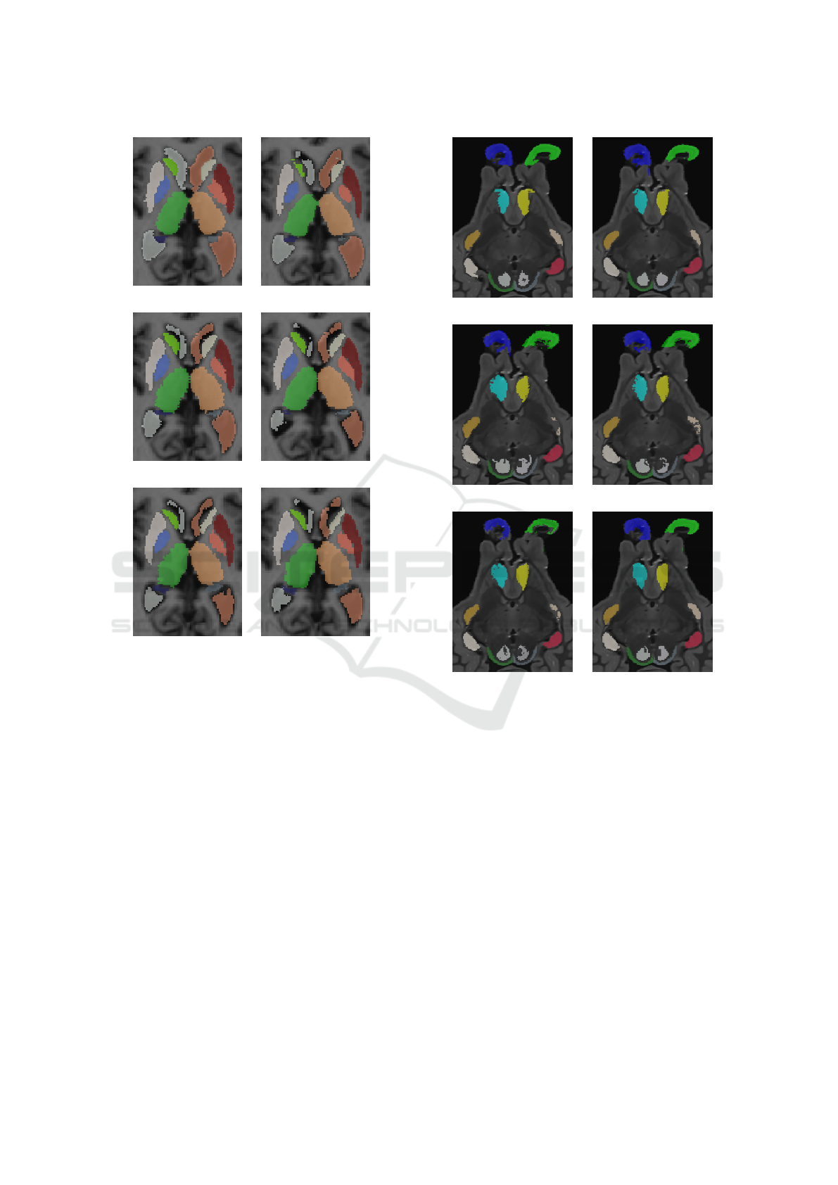
(a) Ground Truth (b) JLF
(c) WV (d) SV
(e) HMF (f) GC
Figure 4: Results of segmentation on the image 1122 for the
experiments E
1
.
ween methods. JLF method which provides the best
segmentations when local atlases are well positioned
is very time consuming compared to all the other met-
hods. In the opposite, only 1 minute is needed by the
GC methods to provide the segmentation of 13 regi-
ons. This computation time is also dependent of the
number of images in the training database. Because
of the registration step, multi-atlas based method (SV,
WV and JLF) are faster if the size of the training da-
tabase is small (and vice versa) which is note the case
of the methods based on probabilistic atlases (HMF
and GC).
5 DISCUSSION
Experiments E
1
and E
2
have been performed without
real user interaction. However the method permits the
intervention of a user in order to correct the position
(a) Ground Truth (b) JLF
(c) WV (d) SV
(e) HMF (f) GC
Figure 5: Results of segmentation on a sheep brain image
of the SheepBrain database for the experiments E
2
.
of a bounding box. In practice, during an interactive
segmentation, the result is close to the one achieve
during the experiment E
1
. Either the automatic posi-
tioning is correct and the user accept it, or the automa-
tic positioning is not correct and the user adjusts the
bounding box. In both case, the final position of the
bounding box before running the classification step is
close to the perfect position. Experiment E
2
described
an automatic way to use the system. The first regions
are well positioned by the user, then the system ends
the segmentation by itself.
The main purpose of this study was to choose the
most suitable segmentation method for a local atlas
segmentation. The final answer is dependent on the
type of utilization that the user wants to perform. Du-
ring an interactive segmentation, the user needs to
have quick visualization of the result which is not pos-
VISAPP 2019 - 14th International Conference on Computer Vision Theory and Applications
348

Table 3: Dice ratio (%) of the E
2
experiment on the MICCAI database. Dice ratio of bilateral anatomical structures have been
averaged.
Structures Brainstem Caud. Nuc. Hippo. Vent. pall. Puta. thal. Average
JLF 78.9 70.5 47.9 75.8 57.7 85.1 89.0 71.5
Weighted Vote 91.4 83.0 80.5 82.5 82.8 89.3 90.7 85.3
Simple Vote 84.43 75.1 56.7 65.1 74.9 85.5 90.4 75.3
HMF 90.1 73.8 69.4 73.0 73.2 85.3 88.1 78.1
GraphCut 75.6 65.3 59.7 62.1 69.1 81.0 88.8 71.3
Table 4: Dice ratio (%) of the E
2
experiment on the SheepBrain database. Dice ratio of bilateral anatomical structures have
been averaged.
Structures Bulb. Olf. Cau. Nuc. Peri. Amyg Inf. Col. Opt. Col. Mot. Col. Hipp. Averag
JLF 8.6 92.1 85.6 77.1 52.6 56.0 43.6 75.8 59.8
WV 41.4 88.2 86.9 77.3 64.9 70.1 50.2 80.9 68.9
SV 10.8 89.5 88.1 75.4 46.0 43.4 36.1 66.4 54.9
HMF 24.0 86.1 87.3 82.4 40.1 46.6 37.4 86.8 59.6
GC 5.4 87.7 88.9 79.6 28.8 28.0 13.6 70.5 47.7
Table 5: Average computation time of segmentation of an
image in the MICCAI database (E1 experiment).
Method Computation time
JLF 418 min
WV 22.4 min
SV 10.9 min
HMF 10.1 min
GC 1.1 min
CNN 5 min
sible to achieve with a JLF segmentation method. GC
and CNN segmentation provide the labeling of a re-
gion in less than 10 seconds which is most suitable
for an interactive process. WV, SV and HMF needs
between 40 seconds and 2 minutes to obtain the seg-
mentation of a region. Even if these methods seem to
provide a better quality than graph-cut segmentation
for the MICCAI database, which is even not the case
for the SheepBrain database, the gap of quality could
not be sufficient to justify their utilization. The time
saved by the GC method can be used to apply a ma-
nual refinement of the segmentation. However a sim-
ple CNN like the one used in this study have shown
some limitations when the training database is small.
If an automatic segmentation is desired, the multi-
atlas method like JLF and weighted voting are more
adapted depending on the time available to perform
the segmentation. These methods provide the more
precise segmentation and can manage the utilization
of the spatial relationships in a better way. In case of
wrong positioning, some of the local atlases can be
wrongly registered. But the weight which is associ-
ated to each atlas in JLF and WV method can limit
the importance of some of the local atlases. Depend-
ing on the difficulty of the situation, these methods
used in an automatic way can be sufficient.
6 CONCLUSION
In this article, six different atlas-based methods for an
interactive and local segmentation of 3D MRI images
have been presented and compared. Each classifica-
tion method have shown to have their own advanta-
ges depending on the variability of the position of the
anatomical structure and the quality of the initial po-
sitioning of the bounding box surrounding the local
region to segment. The usage mode of the segmenta-
tion tool will justify the final choice. The segmenta-
tion of simple regions in an interactive way will lead
to the utilization of fast segmentation processes like
GC. Difficult regions in an automatic way will lead to
more robust segmentation like local weighted majo-
rity voting.
ACKNOWLEDGEMENTS
This work is part of NeuroGeo project and has been
funded by the ”Region Centre Val de Loire - France”.
The authors thank Cyril Poupon (Neurospin, CEA Sa-
clay, France) and Hans Adriaensen (CIRE platform,
Inra Val de Loire, France) for providing the diffe-
rent sheep brain MR images used during these experi-
ments; Ophelie Menant for the manual segmentation
of the NeuroGeoEx database.
A Comparative Study on Voxel Classification Methods for Atlas based Segmentation of Brain Structures from 3D MRI Images
349

REFERENCES
Ashburner, J. and Friston, K. J. (2005). Unified segmenta-
tion. NeuroImage, 26(3):839 – 851.
Boykov, Y. and Kolmogorov, V. (2004). An experimen-
tal comparison of min-cut/max-flow algorithms for
energy minimization in vision. IEEE Trans. Pattern
Anal. Mach. Intell., 26(9):1124–1137.
Boykov, Y., Veksler, O., and Zabih, R. (2001). Fast ap-
proximate energy minimization via graph cuts. IEEE
Transactions on Pattern Analysis and Machine Intel-
ligence, 23(11):1222–1239.
Cabezas, M., Oliver, A., Llad, X., Freixenet, J., and Cua-
dra, M. B. (2011). A review of atlas-based segmenta-
tion for magnetic resonance brain images. Computer
Methods and Programs in Biomedicine, 104(3):e158
– e177.
C¸ ic¸ek,
¨
O., Abdulkadir, A., Lienkamp, S. S., Brox, T., and
Ronneberger, O. (2016). 3d u-net: Learning dense
volumetric segmentation from sparse annotation. In
Ourselin, S., Joskowicz, L., Sabuncu, M. R., Unal,
G., and Wells, W., editors, Medical Image Computing
and Computer-Assisted Intervention – MICCAI 2016,
pages 424–432, Cham. Springer International Publis-
hing.
Dangi, S., Cahill, N., and Linte, C. A. (2017). Integrating at-
las and graph cut methods for left ventricle segmenta-
tion from cardiac cine mri. In Mansi, T., McLeod, K.,
Pop, M., Rhode, K., Sermesant, M., and Young, A.,
editors, Statistical Atlases and Computational Models
of the Heart. Imaging and Modelling Challenges, pa-
ges 76–86, Cham. Springer International Publishing.
Galisot, G., Brouard, T., Ramel, J., and Chaillou, E. (2017).
Image segmentation using local probabilistic atlases
coupled with topological information. In Proceedings
of the 12th International Joint Conference on Compu-
ter Vision, Imaging and Computer Graphics Theory
and Applications (VISIGRAPP 2017) - Volume 4: VI-
SAPP, Porto, Portugal, February 27 - March 1, 2017.,
pages 501–508.
Iglesias, J. E. and Karssemeijer, N. (2009). Robust initial
detection of landmarks in film-screen mammograms
using multiple ffdm atlases. IEEE Transactions on
Medical Imaging, 28(11):1815–1824.
Iglesias, J. E. and Sabuncu, M. R. (2015). Multi-atlas seg-
mentation of biomedical images: A survey. Medical
Image Analysis, 24(1):205 – 219.
Isgum, I., Staring, M., Rutten, A., Prokop, M., Viergever,
M. A., and van Ginneken, B. (2009). Multi-atlas-
based segmentation with local decision fusionappli-
cation to cardiac and aortic segmentation in ct scans.
IEEE Transactions on Medical Imaging, 28(7):1000–
1010.
Klein, A., Mensh, B., Ghosh, S., Tourville, J., and Hirsch, J.
(2005). Mindboggle: Automated brain labeling with
multiple atlases. BMC Medical Imaging, 5(1):7.
Landman, B. A., Warfield, S. K., Hammers, A., Akhondi-
asl, A., Asman, A. J., Ribbens, A., Lucas, B., Avants,
B. B., Ledig, C., Ma, D., Rueckert, D., Vandermeu-
len, D., Maes, F., Holmes, H., Wang, H., Wang, J.,
Doshi, J., Kornegay, J., Hajnal, J. V., Gray, K., Collins,
L., Cardoso, M. J., Lythgoe, M., Styner, M., Armand,
M., Miller, M., Aljabar, P., Suetens, P., Yushkevich,
P. A., Coupe, P., Wolz, R., and Heckemann, R. A.
(2012). MICCAI 2012 Workshop on Multi-Atlas La-
beling. Technical report.
Nitzsche, B., Frey, S., Collins, L. D., Seeger, J., Lobsien,
D., Dreyer, A., Kirsten, H., Stoffel, M. H., Fonov,
V. S., and Boltze, J. (2015). A stereotaxic, population-
averaged t1w ovine brain atlas including cerebral mor-
phology and tissue volumes. Frontiers in Neuroana-
tomy, 9:69.
Platero, C., Tobar, M. C., Sanguino, J., and Velasco, O.
(2014). A new label fusion method using graph
cuts: Application to hippocampus segmentation. In
Roa Romero, L. M., editor, XIII Mediterranean Con-
ference on Medical and Biological Engineering and
Computing 2013, pages 174–177, Cham. Springer In-
ternational Publishing.
Rohlfing, T., Brandt, R., Menzel, R., and Maurer, C. R.
(2004). Evaluation of atlas selection strategies for
atlas-based image segmentation with application to
confocal microscopy images of bee brains. NeuroI-
mage, 21(4):1428 – 1442.
Ronneberger, O., Fischer, P., and Brox, T. (2015). U-net:
Convolutional networks for biomedical image seg-
mentation. In Navab, N., Hornegger, J., Wells, W. M.,
and Frangi, A. F., editors, Medical Image Computing
and Computer-Assisted Intervention – MICCAI 2015,
pages 234–241, Cham. Springer International Publis-
hing.
Scherrer, B., Forbes, F., Garbay, C., and Dojat, M. (2009).
Distributed local mrf models for tissue and structure
brain segmentation. IEEE Transactions on Medical
Imaging, 28(8):1278–1295.
Shattuck, D. W., Mirza, M., Adisetiyo, V., Hojatkashani,
C., Salamon, G., Narr, K. L., Poldrack, R. A., Bilder,
R. M., and Toga, A. W. (2008). Construction of a 3d
probabilistic atlas of human cortical structures. Neu-
roImage, 39(3):1064 – 1080.
Wang, H., Suh, J. W., Das, S. R., Pluta, J. B., Craige, C., and
Yushkevich, P. A. (2013). Multi-atlas segmentation
with joint label fusion. IEEE Transactions on Pattern
Analysis and Machine Intelligence, 35(3):611–623.
Xabier Artaechevarria, Arrate Muoz-Barrutia, C. O.-d.-S.
(2008). Efficient classifier generation and weigh-
ted voting for atlas-based segmentation: two small
steps faster and closer to the combination oracle.
Proc.SPIE, 6914:6914 – 6914 – 9.
VISAPP 2019 - 14th International Conference on Computer Vision Theory and Applications
350