
Energy-Based Visualization of 2D Flow Fields
Karsten Hanser, Stefan Meggendorfer, Peter H¨ugel, Florian Fallenb¨uche l, Hafiz Muhammad Fahad
and Filip Sadlo
IWR, Heidelberg University, Im Neuenheimer Feld 205, H ei delberg, Germany
sadlo@uni-heidelberg.de
Keywords:
Flow Visualization, Bernoulli’s Principle, Energy Conversion.
Abstract:
In this paper, we present a novel approach for energy-based flow visualization. Inspired by Bernoulli’s prin-
ciple, which is limited to steady inviscid flow, we derive a set of energies whose sum is conserved along
pathlines in 2D time-dependent viscous flow. We present an interactive approach for visual analysis based on
these quantities, as well as a compact color-coded representation. This enables effective analysis of energy
conversion along selected pathlines, as well as its spatial coherence. We exemplify the util ity of our approach
using results from computational fluid dynamics and flow in elastic porous media.
1 INTRODUCTION
Many problems in science and engineering require
vector field rep resentations. A prominent example are
flow problems, which are often addressed by compu-
tational fluid dynamics (CFD) by means of numerical
solution of the Navier–Stokes (NS) equations.
There exists a wide spectrum of flow visualization
techniques for analyzing vector field s f rom CFD. On
the one hand, there are geometric approaches, such as
arrow glyphs a nd streamlines, which show the over-
all structure of a flow, but fail at revealing underlying
physical mechanisms. On the other h a nd, there are
physically based approac hes, such as the λ
2
vortex
criterion, which often involve derivatives of the vec-
tor fields and sometimes additional q uantities such as
the pressure field. Either way, most flow visualization
techniques aim at a simplified representation of flow,
often providing a “segmentation” into region s of si-
milar behavior or extraction of respective bou ndaries.
In this paper, we investigate the analysis of flow
fields with regard to their immanent energies. We pre-
sent an approach that, on the one hand, enab les the
analysis of energy conversion in flows for a better un-
derstandin g of the involved phy sical mechan isms. On
the other hand, our approach enables the identification
of regions of physically similar b e havior with respect
to these energies. Our approach is in spired by Ber-
noulli’s principle, which, however, is ap plicable only
to inviscid stationary flow. We extend it to viscous
time-dependent flow, and derive from it a technique
for interactive visual analysis of flow fields.
The contributions of this paper include:
• a set of energy quantities whose sum is conserved
along trajector ies, up to solver-induced err or,
• an approach to quantify that solver-induced e rror
and relate it to our quantities,
• an interactive exploration approach enabling de-
tailed analysis of energy conversion and the phy-
sical mechanisms along trajectories, and
• an approach to reveal the regions of qualitatively
similar behavior with respect to energy dynamics.
2 RELATED WORK
The most closely related work in the field of fluid
dynamics is Bernoulli’s Hydrodynamica (Bernou lli,
1738), which presents the concept later denoted Ber-
noulli’s principle, detailed in Section 3.
Previous work in the context of energy -based flow
visualization includes proper orthogonal decomposi-
tion for separating different scales with respect to
energy (Pobitzer et a l., 2011), and a graph b ased ap-
proach , which focuses on the conversion and trans-
portation of internal and kinetic energy (Fernandes
et al., 2017). The focus of our work, in contrast, is
on decomposition, transport, and conversion of diffe-
rent energy types along pathlines.
Less closely re la ted are physically based criteria,
such as λ
2
(Jeong and Hussain, 1995 ) for vortex ex-
traction, and interaction betwe en shear flow and vorti-
250
Hanser, K., Meggendorfer, S., Hügel, P., Fallenbüchel, F., Fahad, H. and Sadlo, F.
Energy-Based Visualization of 2D Flow Fields.
DOI: 10.5220/0007359602500258
In Proceedings of the 14th International Joint Conference on Computer Vision, Imaging and Computer Graphics Theory and Applications (VISIGRAPP 2019), pages 250-258
ISBN: 978-989-758-354-4
Copyright
c
2019 by SCITEPRESS – Science and Technology Publications, Lda. All rights reserved
ces (Schafhitzel et al., 2011; Sadlo et al., 2006). Other
approa c hes emp loy physical principles for visualizing
advection properties, such as schlieren flow visuali-
zation (Brownlee et al., 2010) and virtual rheoscopic
fluids (Barth a nd Burns, 2007).
3 BERNOULLI’S PRINCIPLE
Bernoulli presented in his early work on hydrodyna-
mics (Bernoulli, 1738) his prin ciple, which r elates ki-
netic, pressure, and potential energy. Assuming invis-
cid steady flow, i.e., flow that has zero viscosity and
no time dependency, his p rinciple states th a t energy is
conserved along streamlines, e.g., if velocity increa-
ses along a streamline, it implies a respective decrease
of pressure energy and/or potential energy. In other
words, it describes the tr ansformatio n of energy along
streamlines in fluid flow.
A streamline
ξ
ξ
ξ
t
x
0
(s) := x
0
+
Z
s
0
u
ξ
ξ
ξ
t
x
0
(σ),t
dσ (1)
is obtain e d by solving a n initial value problem (IVP)
in a single time step t of the (potentially unsteady ) n -
dimensional vector field u(x,t) defined on a domain
Ω ⊆ R
n
, with x ∈ Ω and u ∈ R
n
. That is, one starts the
integration at a seed point x
0
∈ Ω with ξ
ξ
ξ
t
x
0
(0) = x
0
,
and in tegrate s a curve tangential to the vector field
u(x,t) for a given duration s, keeping physical time t
fixed. On the other hand, a p athline
ξ
ξ
ξ
x
0
,t
0
(t) := x
0
+
Z
t
t
0
u(ξ
ξ
ξ
x
0
,t
0
(τ),τ) dτ (2)
is obtained by solving an IVP “including” physical
time, i.e., by starting integration at a seed point x
0
and
seed time t
0
, and integrating along th e time-dependent
vector field u(x,t), that is, the integration parameter
is physical time t. Notice, that in steady vector fields,
streamlines and pathlines are identical.
According to Ber noulli’s principle, along such
a streamline in steady inviscid flow, i.e., at each
point x = ξ
ξ
ξ
t
x
0
(s), the sum of kinetic energy
E
u
(x,t) :=
ku(x,t)k
2
2
, (3)
pressure energy
E
p
(x,t) :=
p(x,t)
ρ
, (4)
and potential energy
E
h
(x) := gh(x), (5)
stays con stant, i.e., E
u
(x,t) + E
p
(x,t) + E
h
(x) =
const., with pressure p(x,t), density of the fluid ρ,
h(x) the height of point x, and gravity g.
(a) u(x,t) (b) E
u
(x,t)
(c) E
p
(x,t) (d) E
t
(x,t)
(e) (f) ε(x,t)
Figure 1: Inviscid steady flow past a back-facing step.
(a) Velocity magnitude (low-black; high-yellow), with stre-
amlines (white). (b) Kinetic energy E
u
(x,t) (low-black;
high-red) is not constant along streamlines, and neither is
pressure energy E
p
(x,t) (c) (low-black; high-blue). (d) To-
tal energy E
t
(x,t) = E
u
(x,t)+E
p
(x,t), however, is constant
up to small deviations. Isolines (red) of E
t
(x,t) and stream-
lines (white and gray) (e) deviate slightly due to inaccura-
cies of the simulation and derivative estimation, which we
quantify as solver error ε(x,t) (f) (0-black; 0.1-magenta).
Figure 1 illustrates the principle, at the example of
a simple inviscid (ν = 0) steady 2D flow simulation
obtained with the G erris flow solver (Popinet, 2007).
In this example (and the following), gravity has been
set to zero for simulation, resulting in zero potential
energy everywhere, i.e., there is only conversion be-
tween kinetic and p ressure energy here. Notice, that
the focus of this paper is flow visualization, i.e., th e
input to our technique is the simulated fields u(x,t),
p(x,t), as well es density ρ and viscosity ν.
It is apparent that E
u
(x,t) (Figure 1(b)) is not uni-
form along the streamlines, and that neither is E
p
(x,t)
(Figure 1(c)). Nevertheless, their sum, which we de-
note total energy E
t
(x,t) := E
u
(x,t) + E
p
(x,t), is al-
most constant (Figure 1 (d)), as can be seen when
comparing the streamlin es to isolines of E
t
(x,t) (Fi-
gure 1(e)). The small deviations between stre amlines
and isolines of E
t
stem f rom inaccuracies of the simu-
lation and d erivative estimation during visualization.
To assess suc h inaccura cies, we derive a quan-
tity which we denote solver error ε(x,t) (Figure 1(f)).
Energy-Based Visualization of 2D Flow Fields
251

The numerical solver aims at solving the NS equation
Du(x,t)
Dt
= −
∇p(x,t)
ρ
+ ν∆u(x,t), (6)
with material derivative
Du(x,t)
Dt
:=
∂u(x,t)
∂t
+ (∇u(x,t))u(x,t), (7)
density ρ, Laplacian ∆, an d kinematic viscosity ν.
However, due to in accuracies (non z ero solver resid u-
als, as well as potential inconsistencies between de -
rivative estimation in the solver and estimation du-
ring our visualization process), the left hand side is in
general not identical to the right hand side when the
terms of Equation 6 are computed from the simulated
fields u(x,t) and p(x,t). This motivates us to obtain ε
as the discrepancy between the two sides, i.e.,
ε(x,t) :=
1
µ
Du(x,t)
Dt
+
∇p(x,t)
ρ
− ν∆u(x,t)
, (8)
normalized by µ, which is the average of the magni-
tude of Du(x,t)/Dt over the domain Ω:
µ :=
1
vol(Ω)
Z
Ω
Du(x,t)
Dt
dΩ, (9)
with vol(Ω) being the volume (a rea) of the domain.
4 METHOD
The majority of fluid dyn a mics pro blems involves
time dependency and necessitates nonzero viscosity,
which strongly limits the applicability of Bernoulli’s
principle. Our main aim in this work, is to ad-
dress both of these issues, i.e., to derive a concept
that en ables energy-based flow visualization in time-
dependent viscous flow. Where a s we formulate our
approa c h here for 2D flows, its extension to 3D dom-
ains would be straightforward in large p arts.
4.1 Derivation of Energies
Let us start with a steady CFD simula tion of a flow
around an obstacle. Again, gravity g was set to
zero for simulation, but in this case, the modeled
fluid has nonzero kinematic viscosity ν, leading to
a wake behind the obstacle exh ibiting low veloci-
ties (Figure 2(a)). The kinetic energy field E
u
(x,t)
(Figure 2(c)) and the pressure energy E
p
(x,t) (Fi-
gure 2(e)) can be easily computed according to Equ a-
tions 3 and 4 using the simula te d fields u(x,t) and
p(x,t). However, if these energies ar e summed up to
obtain the total energy E
t
(x,t), the resulting field (Fi-
gure 2(g)) is not constant along streamlines, in con-
trast to the inviscid ca se from Section 3 (Figure 1(d)).
The rea son for this discr e pancy is the nonz ero vis-
cosity, which is violating the assumption s of Ber-
noulli’s principle. That is, velocity undergo e s diffu-
sion due to the viscosity (according to the rightmost
term ν∆u(x,t) in Equation 6). In other words, the
internal friction in the flow “ tries to minimize” the
gradient of the velocity field and thu s causes kinetic
energy to “diffuse”. The direction of this diffusion is
not constrained to directions along streamlines, and
therefore E
t
is, in general, no t constant along a stre-
amline in viscous flow.
An interesting observation is, however, that since
the Navier–Stokes eq uation (Equation 6) represents
the materia l derivative of velocity u(x,t), it descri-
bes the acceleration of a fluid parcel at location x and
time t. On the other hand, Bernoulli’s pr inciple invol-
ves the variation of k inetic energy E
u
along a stream-
line. The difference of kinetic energy be tween two
points s
0
and s
1
on such a strea mline has to equal
the total work between these points, and sin ce work
equals the integral of force along a path, we obtain
E
u
(x
1
,t) = E
u
(x
0
,t) +
Z
s
1
s
0
Du(ξ
ξ
ξ
t
x
0
(s),t)
Dt
·ds, (10)
with x
0
= ξ
ξ
ξ
t
x
0
(s
0
) and x
1
= ξ
ξ
ξ
t
x
0
(s
1
) being the re-
spective positions on the streamline, and line ele-
ment ds := u(ξ
ξ
ξ
t
x
0
(s),t)ds. Notice th at E
u
is a specific
energy in Berno ulli’s formulation, and therefore we
do not need to multiply the material derivative with
density ρ to obtain E
u
(x
1
,t). Notice also that since
pathlines and streamlines are ide ntical in steady flow,
and since the Navier–Stokes equation also holds for
unsteady flow, we can replac e in Equation 10 the stre-
amline ξ
ξ
ξ
t
x
0
by a pathline ξ
ξ
ξ
x
0
,t
0
in this example (and in
general, as we will see la ter).
Altogether, Equation 10 provides an alternative
approa c h for computing E
u
(x,t), i.e., at time t, we
can start a pathline at point x, integrate it bac kward
in time (in reverse flow direction) until time t
α
(with
t
α
< t), and evaluate th e line integral accordingly:
˜
E
u
(x,t) = C
u
+
Z
t
α
t
Du(ξ
ξ
ξ
x,t
(τ),τ)
Dt
·dτ
τ
τ, (11)
with line element dτ
τ
τ := u(ξ
ξ
ξ
x,t
(τ),τ)dτ, and pathline
ξ
ξ
ξ
x,t
(τ) := x +
Z
τ
t
u(ξ
ξ
ξ
x,t
(τ),τ) dτ (12)
with τ < t. C
u
is an integration constant, which needs
to be chosen. Notice that we denote our result in tegra-
ted kinetic energy
˜
E
u
, in contrast to Bernoulli’s kinetic
energy E
u
.
Figure 2(d) shows
˜
E
u
(x,t) for C
u
= 0, with re-
verse integration duratio n of 100 seconds. For this
integration duration, the pathlines either reach th e in-
let at the left boundary, or stay in the recirculation
IVAPP 2019 - 10th International Conference on Information Visualization Theory and Applications
252
(a) u(x,t)
(b)
˜
E
ν
(x,t)
(c) E
u
(x,t)
(d)
˜
E
u
(x,t)
(e) E
p
(x,t)
(f)
˜
E
p
(x,t)
(g) E
t
(x,t)
(h)
˜
E
t
(x,t)
Figure 2: Steady viscous flow around obstacle, from left to right. (a) Velocity u(x) together with streamlines (w hit e). (b) In-
tegrated diffusion energy
˜
E
ν
(x), according to Equation 15, with two selected streamlines (gray). (c) Kinetic energy E
u
(x),
computed locally according to Equation 3. ( d) Integrated kinetic energy
˜
E
u
(x) (Equation 11). (e) Pressure energy E
p
(x)
and (f) integrated pressure energy
˜
E
p
(x,t) (Equation 14). (g) Total energy E
t
(x) is not conserved along streamlines, whereas
integrated total energy
˜
E
t
is, i.e.,
˜
E
u
+
˜
E
p
+
˜
E
ν
= const. is our counterpart to Bernoulli’s principle for unsteady viscous flow.
region right to the obstacle. Since the in le t velo-
city is constan t along the inlet, Figure 2(d) is, up
to an additive constant, identical to Figure 2(c ), ex-
cept for the region behind the obstacle. The reason
why
˜
E
u
(x,t) in that region h as values different from
E
u
(x,t), is that setting C
u
= 0 there is not consistent
with setting C
u
= 0 at the inlet. While one co uld set
C
u
= E
u
(ξ
ξ
ξ
−
x,t
(t
α
)), i.e., to the value of E
u
at the “up-
stream end” of the pathline, such an evaluation cannot
be ac hieved for our integrated diffusion energy intr o-
duced below. Therefore, we set C
u
= 0.
If we bring the right hand side of Equation 6 to
the left side, we have three terms on th e left hand side
that su m up to zero, i.e.,
Du(x,t)
Dt
+
∇p(x,t)
ρ
− ν∆u(x,t) = 0, (13)
or, in other words, thr ee terms whose sum is constant
along a pathline.
The same procedure as for
˜
E
u
(x,t) can be car ried
out with respect to the pressure term, leading to the
integrated p ressure ene rgy
˜
E
p
(x,t) = C
p
+
Z
t
α
t
∇p(ξ
ξ
ξ
−
x,t
(τ),τ)
ρ
·dτ
τ
τ. (14)
For the same reasons a s above, we set C
p
= 0, which
results in Figure 2(f).
In analogy, the third term of Equ a tion 13 moti-
vates to compute the energy difference between two
points along a pathline due to energy diffusion as:
˜
E
ν
(x,t) = C
ν
−
Z
t
α
t
ν∆u(ξ
ξ
ξ
−
x,t
(τ),τ)· dτ
τ
τ, (15)
which we deno te integrated diffusion energy (Fi-
gure 2(b)). Notice that
˜
E
ν
cannot be obtained without
Energy-Based Visualization of 2D Flow Fields
253
(a) (b)
Figure 3: 2D pathline plots, with
˜
E
u
(red),
˜
E
p
(blue),
˜
E
ν
(green),
˜
E
t
(yellow), and ε (gray). ( a) Pl ot corresponding to
upper selected (gray) streamline in Figure 2. (b) Plot corre-
sponding to lower selected (gray) streamline in Fi gure 2.
integration, whereas E
u
and E
p
could. Nevertheless,
for consistency, we will work with
˜
E
u
,
˜
E
p
, and
˜
E
ν
.
Finally,
˜
E
t
(x,t) :=
˜
E
u
(x,t) +
˜
E
p
(x,t) +
˜
E
ν
(x,t),
our integrated total energy, is conserved along pathli-
nes, and represents the basis for our approach. It can
be seen as the counterpart to Bernoulli’s principle, for
unsteady viscous flow. Figure 2(h) shows
˜
E
t
, and one
can see that the field is c onstant along pathlines, in
contrast to E
t
(Figure 2(g )).
4.2 2D Pathline Plots
To ease visual analysis of the variation (conversion)
of the energies
˜
E
u
,
˜
E
p
, and
˜
E
ν
along path lines, we
introdu ce 2D pathline plots. In these plots, a given
pathline represents the abscissa, parametrized by arc
length in flow direction. Figure 3(a) shows th e plot fo r
the uppe r gray pathline (which is identical to a stre-
amline in this case) in Figure 2, whereas Figure 3(b)
shows the plot for the lower gray pathline in Figure 2.
In our implementation, the user can interactively seed
a pathline and explore the transformation of energy
along it by examining the respective plot in a linked
view. It can be seen how the energies are converted
and that
˜
E
t
is indeed conserved .
The upper pathline (Figu re 3(a)) passes close by
the obstacle. Befor e the obstacle,
˜
E
u
reduces an d
˜
E
p
increases, indicating conversion from kinetic to pr es-
sure energy. Beh ind the obstacle (where the pathline
resides in the low-velocity wake),
˜
E
u
is low but incre-
asing, while
˜
E
ν
is decaying almost at the same rate,
whereas
˜
E
p
stays almo st constant. This in dicates that
kinetic energy is transported from the outside into this
region by diffusion, which means that that part of the
wake is accelerated due to viscosity, but influenced by
pressure only in close vicinity to th e obstacle.
Energy dynam ics alo ng the lower pathline (Fi-
gure 3( b)), on the other hand, is ba sically not af -
fected by viscosity. We identify from the pathline
plot that the flow is first accelerated due to conver-
sion from pressure energy to kin e tic energy, and la-
(a)
˜
E
u
(b)
˜
E
p
(c)
˜
E
ν
(d)
˜
E
t
(e)
Figure 4: 3D pathline plots provide context for the 2D
pathline plots. The front gray pathline corresponds to Fi-
gure 3(b), whereas the farther one refers to the plot form
Figure 3(a). For more compact context, the surfaces can be
combined into a single view (e).
ter the flow decelerates again, by transformin g kinetic
energy back to pressure energy.
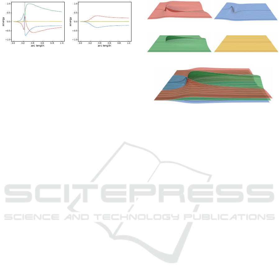
4.3 3D Pathline Plots
Whereas the 2D pathline plots are an effective me-
ans for interactive analysis of energy dynamics al-
ong individual pathlines, they do not provide context,
i.e., they do not give information about the relation or
compariso n between different pathlines. To this end,
we introduce 3 D pathline p lots, as a complementary
technique that provides overview and context. We
construct these plots by computing a rake of pathlines
(i.e., a set of pa thlines seeded along a straight seeding
curve, e.g., as shown in Figure 2), generating the 2D
plot f or each of these pathlines, and then creating a
mesh betwe e n “adjace nt” curves of the same quantity.
That is, we take for each of the quantities
˜
E
u
,
˜
E
p
,
˜
E
ν
and
˜
E
t
all arc-length parametrized cu rves, distribute
them evenly in “orthogonal” direction, and cre a te for
each of the quantities a triangle mesh. Figure 4(a)–(d)
shows an example for th e resulting surfaces. Notice
that in Figure 2, we show only every second pathline
that is used for generating the 3D plots, and for better
visibility, we additiona lly show only the lower half.
For improved context, the selected 2D pathline is
denoted b y a dark gray curve both in the 2D fields, as
well a s on the 3D plot surfaces. For more compact
overview, the resulting surfaces can also be merged
(Figure 4(e)), h owever, in that configuration they rat-
her serve for context than for qualitative insights, due
to potential occlusion issues and clutter.
IVAPP 2019 - 10th International Conference on Information Visualization Theory and Applications
254
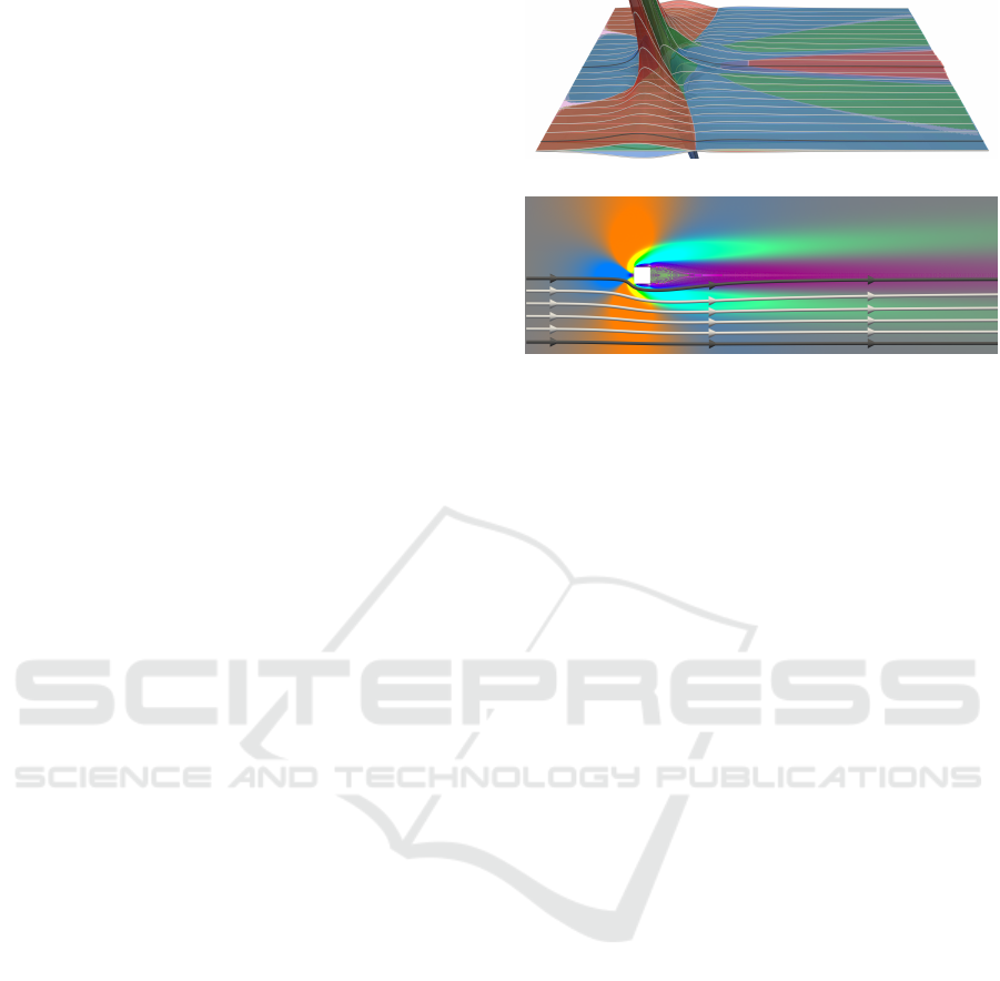
4.4 Energy Conversion Maps
Although the 3D pa thline plots provide g ood context
for interactive exploration by means of 2D pathline
plots, they exhibit several shortcomings for qualita-
tive or even quantitative analysis.
First, as mentioned above, their merged represen-
tation (Figure 4(e)) ten ds to suffer from occlusion and
visual clutter. Second, the fact tha t they do not re-
present the sp atial domain but instead a space that is
spanned by pathline arc length and pathline index hin-
ders interpretation. Third, we set the constants C
u
,
C
p
, and C
ν
to zero, but any choice would be possi-
ble, which ma kes the “offset height” of the individual
pathline curves in the 3D pathline plot surfaces ba-
sically m e aningless, including their intersectio n (e.g.,
the intersection between the red and green manifold
in Fig ure 4(e )). Since the final goal of o ur work is the
analysis of conversion of different ty pes of energy, it
is rather the rate of change of these energies along a
pathline that is of interest, than their value itself. This
motivates us to use material derivatives of
˜
E
u
,
˜
E
p
, and
˜
E
ν
for a more qualitative and quantitative analysis.
The mate rial derivative is a differentiation with re-
spect to tim e -dependent flow, and it cap tures the rate
of change of a quantity, as “observed” alo ng a path-
line. Th us, the material derivative of
˜
E
u
,
˜
E
p
, and
˜
E
ν
gives us the amount of energy type per time unit that is
gained or lost by means of energy conversion along a
pathline. We could plot these derivatives again by me-
ans of the 3D pa thline plot approach (see Fig ure 5(a)
for an example). Whereas this would solve the issue
with the constants, since they vanish in the deriva-
tive, this representation would still suffer from occlu-
sion, visual clutter, and non -spatial domain. The re-
fore, we present energy conversion maps, our final
component that complements our already presented
building blocks.
Our energy conversion maps are 2D RGB image s
in c ase of 2D flow. For
˜
E
u
, we compute its mate-
rial derivative D
˜
E
u
(x,t)/Dt, determine the 5th per-
centile P
5
and the 95th percentile P
95
of the material
derivative, obtain the maximum P
m
of |P
5
| a nd |P
95
|,
and then linearly map the material derivative to the
red channel, mapping −P
m
to zero red value and P
m
to full red value. Analogously, we map the material
derivative of
˜
E
ν
to the green channel, and the mate-
rial derivative of
˜
E
p
to the blue channe l. This means,
that if all material derivatives are zero, this will result
in medium gray co lor. Figure 5(b) shows a respective
result, correspo nding to Figure 5(a).
The light blue region in front of the obstacle in
Figure 5(b), for example, corresp onds to conversion
of k inetic to pressure ene rgy. The o range region to
(a)
(b)
Figure 5: (a) 3D plot representation of material derivat ives
of
˜
E
u
(red),
˜
E
p
(blue), and
˜
E
ν
(green). (b) Energy conver-
sion map, mapping to red, green, and blue color channel.
the sides of the obstacle, on the othe r hand, indicates
conversion of pressure energy to kinetic energy. The
purple region behind the obstacle, i.e., in its wake, re-
presents conversion from diffusion energy to both ki-
netic and pressure energy. Finally, the greenish parts
on either side of the purple wake in dicate conversion
from kinetic and pressure energy to diffusion energy,
which means that the greenish regions “give” their
energy to the purple one via viscous interaction .
5 RESULTS
Having in place our overall technique, we will ap-
ply it now to different datasets. First, we exa-
mine a slightly time-dependent flow around an obsta-
cle (Section 5.1), followed by a more unsteady case
exhibiting a K´arm´an vortex street (Section 5.2). Fi-
nally, we demonstrate that our approach is also ap-
plicable to advanced flow problems, suc h as the flow
through elastic porou s media (Section 5.3).
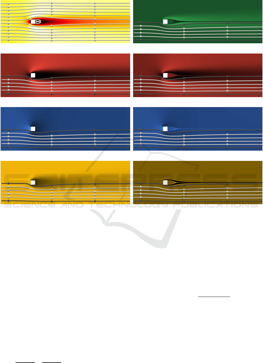
5.1 Slightly Unsteady Obstacle Flow
We now exam ine a CFD simulation tha t has been si-
mulated on the same geometry as the above steady
obstacle flow, but with higher inlet velocity. As a
consequence, the flow is slightly time-dependent, i.e.,
the wake behind the obstacle is “oscillating”. Fi-
gure 6(a) shows streamline s of a snapshot of the time-
dependent flow, whereas Figure 6(b)–(e) show the
pathlines used for plot-b a sed visualization. Notice
that
˜
E
u
,
˜
E
p
,
˜
E
ν
, and
˜
E
t
are not consistent with the
pathlines, since these fields are computed by a large
set of reverse-integrated pathlines started at each point
Energy-Based Visualization of 2D Flow Fields
255
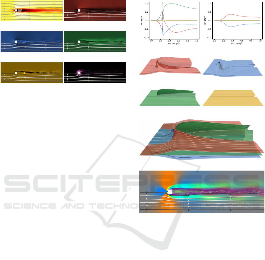
(a) u(x,t)
(b)
˜
E
u
(c)
˜
E
p
(d)
˜
E
ν
(e)
˜
E
t
(f) ε
Figure 6: Slightly unsteady obstacle flow. (a) Velocity
magnitude with streamlines. (b) Integrated kinetic energy
with pathlines (white and gray). (c) Integrated pressure
energy. (d) Integrated diffusion energy. (e) Integrated to-
tal energy. (f) Solver error.
in space, as explained above, and therefore are loca-
ted at different space -time location. Nevertheless, a
look at the respective pathline plots (Figure 7(a) f or
the upper gray pathline an d Figure 7(b) fo r the lower
one) reveals that
˜
E
t
is still conserved very well along
these pathlines. A closer inspection of Figure 7(a) re-
veals that
˜
E
t
slightly increases when the pathline pas-
ses the obstacle. This is consistent w ith higher va-
lues of the solver error ε the re. Overall, investiga-
ting the 3D pathline plots (Figure 7(c)–(g)) and the
energy conversion m ap (Figure 7(h)) reveals that this
flow is still similar to the steady one from Section 4,
and tha t our a pproach works equally well with pathli-
nes in time-depe ndent flow.
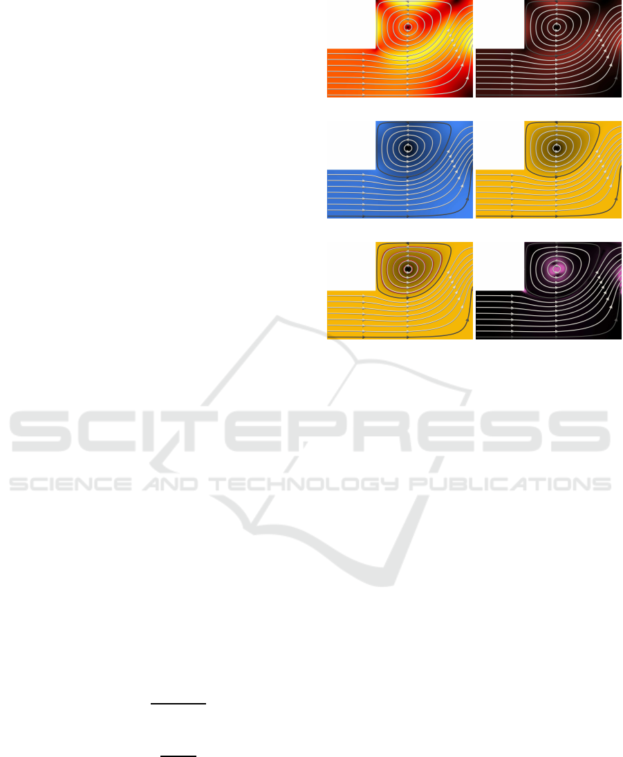
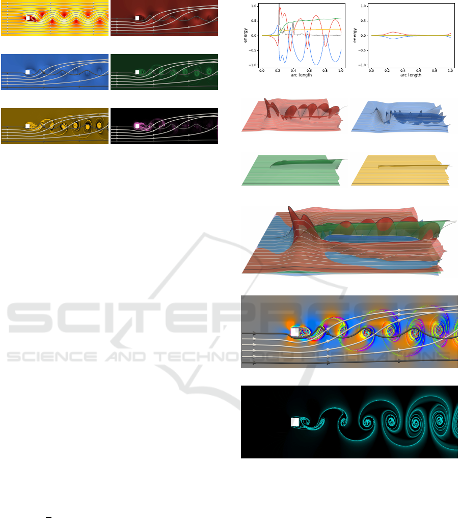
5.2 K
´
arm
´
an Vortex Street
This example is the result of increasing the inlet velo-
city even more, resultin g in K´arm´an vortex sh edding.
As can be seen from the different energy fields and
the comparison between streamlines (Figure 8(a)) and
pathlines (Figure 8(b)–(e )), this dataset is substan-
tially time-dependent. Furthermore, it exhibits lar-
ger solver erro r ε (Figure 8(f)) than the one from
Section 5.1. This larger error leads to a lower level
of energy conservation at the obstacle, as c a n be seen
from the variation of
˜
E
t
in the 2D pathline plot for
the uppe r pathline (Figure 9(a)). In contrast, energy
is well conserved for the lower pathline (Figure 9(b)),
consistent with the lower solver err or in that region.
The energy conversion map (Figure 9(h)) reveals
that the area around the vortex shedding is domina-
ted by c onversion from kinetic to pressure energy
(light blue ), and back fr om pressure energy to kine-
tic energy (orange). Close to the Lagrangian coherent
(a) (b)
(c)
˜
E
u
(d)
˜
E
p
(e)
˜
E
ν
(f)
˜
E
t
(g)
(h)
Figure 7: Slightly unsteady obstacle flow. 2D pathline plot
for upper ( a) gray pathline from Figure 6(b) and lower (b)
one. 3D pathline plots (c)–(g). (h) Energy conversion map
reveals similarity with steady example from Section 4.
structures (ridges in the reverse finite-time Lyapunov
exponent field (Figure 9(i)), computed for the same
integration time as our energies), our approach in dica-
tes conversion from kinetic and pressure energy to dif-
fusion energy (green) , and b ack from diffusion energy
to kine tic and pressure energy (purple). This may
indicate, similar to the case from Figure 5(b), that
energy is transported via viscous mechanisms (diffu-
sion). Besides that, the dark blue regions indicate co n-
version from kinetic and diffusion energy to pressure
energy, and the yellow regions back from pressure to
kinetic and diffusion energy, also re la ting to viscous
effects. Nevertheless, a more deta iled analysis and va-
lidation regarding the impact of ε has to be subject to
future work.
IVAPP 2019 - 10th International Conference on Information Visualization Theory and Applications
256
(a) u(x,t)
(b)
˜
E
u
(c)
˜
E
p
(d)
˜
E
ν
(e)
˜
E
t
(f) ε
Figure 8: K´arm´an dataset. (a) Velocity magnitude with
streamlines (white). Kinetic (b), pressure (c), diffusion (d),
and total energy (e). Solver error (f) is considerably higher
compared to the slightly unsteady case (Figure 6(f)).
5.3 Elastic Porous Flow
Our last example is a simulation of a flow through an
elastic porous medium. In this case, it is the solution
of the consolidation mode l of Biot, which averages
the porous medium to macroscopic scale. The setup,
which is quadratic in rest state, exhibits three diffe-
rent permeabilities (Figure 11(a)). The upper and lo-
wer boundaries are non-pe rmeable, the left boundary
is a velocity inlet, and the right boundary serves as a
“valve”, i.e., the permeability is very low during the
first phase, and high during the second phase. As a
consequence, the material is first “inflated”, and starts
releasing the fluid after the inflow has been stopped
and the right boundary has been “opened”.
Since this example consists of an elastic porous
medium, within which e nergy can be stored as pres-
sure and deformation, we replace the material deriva-
tive of ene rgies by the time derivative, i.e., we focus
on the ma te rial instead of the flow through the mate-
rial. Also, due to the used simulation model, we do
not need to take into account diffusion caused by vis-
cosity. Thus, diffusion energy from above is replaced
by deformation energy, which we compute a s
E
d
:=
1
2
Z
C
k∇d(x,t) + (∇d(x,t))
⊤
k
2
dx
+
Z
C
|∇· d(x,t)|
2
dx,
(16)
with displacement field d(x,t) and cell C of the grid.
Figure 10(a)–(c) shows the first phase o f the pro-
cess for kinetic energy, (f)–(h ) for pressure energy,
and (k)–(m) deformation energy. Accordingly, (c) –(e)
shows the second phase for kinetic e nergy, (h) –(j) for
pressure energy, and (m)–(o) for deformation energy.
Figure 11(b) d epicts energy dynamics at the c e nter.
(a) (b)
(c)
˜
E
u
(d)
˜
E
p
(e)
˜
E
ν
(f)
˜
E
t
(g)
(h)
(i)
Figure 9: K´arm´an fl ow. 2D pathline plots (a) and (b) reveal
that energy conservation is violated close to the obstacle due
to high solver error (Figure 8(f)) in that region. 3D pathline
plots (c)–(g) r eflect energy dynamics of vortex shedding.
(h) Energy conversion map. (i) Finite-time Lyapunov expo-
nent field, for comparison (low-black; high-cyan).
The th ree ph a ses and respective energy conversions
are clearly visible in the plo t. It is appar ent that du-
ring the inflation phase, kinetic en e rgy is higher at
the inlet, whereas during the outflow ph ase, kinetic
energy is larger at the o utlet. Interestingly, pressure
energy as well as deformation energy a re larger at the
inlet in both phases. The energy conversion maps (Fi-
gure 10(p)–(t)), based on the time derivative, reveal
Energy-Based Visualization of 2D Flow Fields
257
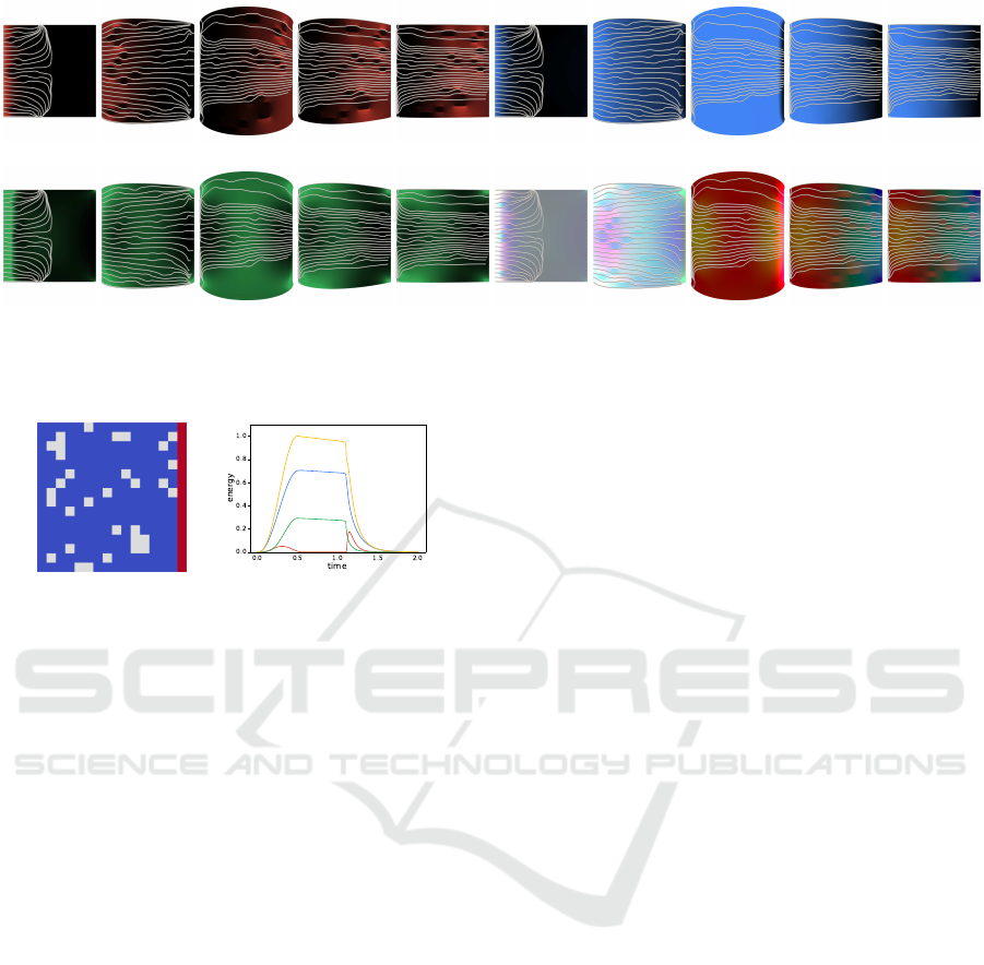
(a) (b) (c) (d) (e) (f) (g) (h) (i) (j)
(k) (l) (m) (n) (o) (p) (q) (r) (s) (t)
Figure 10: Elastic porous flow. (a)–(e) Kinetic energy, (f)–(j) pressure energy, (k)–(o) deformation energy, and (p)–(t) re-
spective energy conversion maps, each wi th respective streamlines.
(a) (b)
Figure 11: Elastic porous flow. (a) High (blue), medium
(gray), and very low (red) permeability. (b) Plot of ki-
netic (red), pressure (blue), deformation (green), and to-
tal (yellow) energy over time, at the center of the domain.
that during the first phase, energy conversion is low
(close to gray colors), whereas at the start of the se-
cond phase, one can see conversion from pressure and
deformation energy to k inetic energy, in p articular at
the outlet. During the second p hase, we observe that
the region that converts deformation and pressure into
kinetic energy shrinks from righ t to left.
6 CONCLUSION
We presented a counterpart to Berno ulli’s principle,
which describes the conservation a nd co nversion of
energy alon g streamlines in inviscid flow. By exten-
ding the concept to time-dependent flow and accou n-
ting for viscous effects, w e established a basis for the
visualization o f energy dynamics in flow fields. We
presented an interactive exploration approach based
on our concept, complemented it with a direct visu-
alization approach of e nergy conversion, and demo n-
strated its utility using simple examples. As future
work, we would like to further investigate the proper-
ties of our appro ach using additional examples, and
extend it to 3D flow fields and other types of energy.
ACKNOWLEDGEMENTS
The research lea ding to these results has been done
within the Transregional Collaborative Research Cen-
ter SFB / TRR 16 5 “Waves to Weather” funded by the
German Science Foundation (DFG).
REFERENCES
Barth, W. and Burns, C. (2007). Virtual rheoscopic fluids
for flow visualization. IEEE Transactions on Visuali-
zation and Computer Graphics, 13(6):1751–1758.
Bernoulli, D. (1738). Hydrodynamica, sive de viribus et
motibus fluidorum commentarii. Opus academicum ab
auctore, dum Petropoli ageret, congestum.
Brownlee, C., Pegoraro, V., Shankar, S., McCormick, P.,
and Hansen, C. (2010). Physically-based interactive
schlieren flow visualization. In Proc. IEEE Pacific Vi-
sualization Symposium 2010, pages 145–152.
Fernandes, O., Frey, S. , and Ertl, T. (2017). Transportation-
based visualization of energy conversion. In P roc.
IVAPP 2017, volume 3, pages 52–63.
Jeong, J. and Hussain, F. (1995). On the identification of a
vortex. Journal of Fluid Mechanics, 285(69):69–94.
Pobitzer, A., Tutkun, M., Andreassen, O., Fuchs, R., Pei-
kert, R., and Hauser, H. (2011). Energy-scale aware
feature extraction for flow visualization. Computer
Graphics Forum, 30(3):771–780.
Popinet, S. (2007). The Gerris flow solver. In Rencontres
Mondiales du Logiciel Li bre, July.
Sadlo, F., Peikert, R., and Sick, M. (2006). Visualization
tools for vorticity transport analysis i n incompressible
flow. IEEE Transactions on Visualization and Com-
puter Graphics, 12(5):949–956.
Schafhitzel, T., Baysal, K., Vaaraniemi, M., Rist, U.,
and Weiskopf, D. (2011). Visualizing the evolution
and interaction of vortices and shear layers in time-
dependent 3D flow. IEEE Transactions on Visualiza-
tion and Computer Graphics, 17(4):412–425.
IVAPP 2019 - 10th International Conference on Information Visualization Theory and Applications
258
