Kohonen Map Modification for Classification Tasks

Jiří Jelínek

Institute of Applied Informatics, Faculty of Science, University of South Bohemia,

Branišovská 1760, České Budějovice, Czech Republic

Keywords: Kohonen Map, Neural Networks, Pattern Classification.

Abstract: This paper aims to present a classification model based on Kohonen maps with a modified learning

mechanism and structure as well. Modification of the model structure consists of its modification for

hierarchical training and recall. The change of the learning process is the transition from unsupervised to

supervised learning. Experiments were performed with the modified model to verify changes in the model

and compare the results with other research.

1 INTRODUCTION

A variety of methods are available for advanced data

processing, often in the field of artificial intelligence.

Their use then depends on what data we have and

what tasks we want to solve. One group of possible

tools for the implementation of machine learning or

data analysis has quite a long been a neural network.

For the learning of neural networks are used two

types of learning methods. In unsupervised learning,

we only have unrated input data that we intend to

analyze in some way. This procedure is typically used

in the early stages of data analysis when we examine

the structure of the data, its internal relationships, and

its character.

In supervised learning, we train the model not

only with the input patterns but also with the required

output. These examples of the R

> R

transformation

are used to form internal rules or model parameter

settings. This approach is suitable for tasks with the

desired transformation function, e.g., classification.

If we use a neural network, our goal is to learn the

network to be able to respond appropriately to inputs

that have not been trained with (the principle of

generalization). Therefore, two disjoint data sets -

training and testing - are typically used. The process

of using the model can thus be divided into two main

phases - the setting phase (learning) and the

production phase (recall). The production phase is the

very reason for the existence of the model, in it, the

learned settings are used for processing of previously

unseen (test) input data.

A useful but nowadays not very frequently used

model is the so-called Kohonen map, which is

designed for unsupervised learning and therefore

cluster data analysis. The big advantage of the model

is a visual representation of network activity.

The author worked with Kohonen maps

previously, and this work showed the weaknesses of

learning algorithms (esp. 2D area fragmentation) and

the limitations of unsupervised learning. On the other

hand, the solved tasks revealed that Kohonen maps

are very comfortable for use in systems with

a required visual representation of learning dynamics.

That was the primary motivation for modifying of

Kohonen network model and extending its

capabilities presented in this paper.

Therefore, a modified learning algorithm and

a multi-level model structure based on Kohonen maps

were designed. The model was experimentally used

(as the proof of concept) for the task of economic data

processing (Vochozka et al., 2017) and preliminarily

tested (Jelínek, 2018). This paper aims to present the

actual state of the model and new experiments with it

to demonstrate its usefulness.

The following chapters are organized as follows.

In Chapter 2 is briefly discussed the related work.

Chapter 3 focuses on a description of the standard

Kohonen map model and shows the parameters of it.

Chapter 4 then concentrates on the description of the

modifications that were made, and Chapter 5 focuses

on experiments with the model conducted primarily

to verify the benefits of the proposed modifications.

584

Jelínek, J.

Kohonen Map Modiﬁcation for Classiﬁcation Tasks.

DOI: 10.5220/0007361405840591

In Proceedings of the 11th International Conference on Agents and Artiﬁcial Intelligence (ICAART 2019), pages 584-591

ISBN: 978-989-758-350-6

2 RELATED WORK

When we talk about neural networks for the

implementation of machine learning or data analysis,

we usually mean a neural network based on an

artificial neuron model (McCulloch and Pitts, 1943).

Probably the greatest attention was given to models

of multi-layered perceptron (Rosenblatt, 1957) and

models based on this principle and using back

propagation method of learning (Rumelhart et al.,

1986).

The multilayer artificial neural network models

have their renaissance nowadays, primarily due to the

deep learning paradigm. This approach enables the

model to learn patterns on a different level of

abstraction. However, our approach is not of this

kind. The deep learning models use the same input set

all the time; our model reduces the set in the course

of the learning process.

A typical example of the slightly different neural

network model with unsupervised learning is the

ART2 algorithm and model (Carpenter and

Grossberg, 1987), which is capable of solving cluster

analysis task, and its operation can be modified by

adjusting the sensitivity of the model to differences in

input data. The higher the sensitivity, the more output

categories or clusters the system creates.

The Kohonen map (Kohonen, 1982) was

introduced in the 1980s as most basic models of

neural networks and is classified into a group of Self-

organizing maps. In some ways, the Kohonen map

can remind us of the ART2 model. The similarity lies

in the same requirements on input data (number

vectors). Similar is also the structure of the network,

which is essentially two-layer. However, Kohonen

map used 2D second layer and is focused on the visual

interpretation of the output and is therefore useful

both for the better understanding of the task and, e.g.,

for use in a dynamic online environment. An example

of such usage can be monitoring the state of the

system and its dynamics (Jelínek, 1992).

We can find also works concentrating on

hierarchical usage of Kohonen maps. In (Rauber et

al., 2002) the hierarchy is constructed dynamically in

the case of clustering very different input patterns into

one output cell. However, our model is based on

supervised learning and uses of extended information

about correct input classification for hierarchical

reduction of the input set. Modification of Self

Organizing Maps for supervised learning based on

RBF is shown in (Fritzke, 1994), our model uses a

different approach to that problem.

3 KOHONEN MAP

The core activity of the Kohonen map is assigning

input patterns to the cells of the second layer (i.e., the

output clusters representing by these cells) based on

the similarity of patterns.

The input layer of the Kohonen map is composed

of the same number of cells as the dimension n of the

input space R

is. The output layer is two-dimensional

and is also referred to as the Kohonen layer. This

structure was chosen concerning output visualization.

The input and output layers are fully interconnected

from the input to the output one with links whose

weights are interpretable as the centroid of the input

patterns cluster represented by the selected cell of the

output layer. The number of output layer cells is the

model parameter.

In the production phase, test patterns are

submitted at the input of the model. Their distance

(here the Euclidean one) is calculated from the output

layer cell centroids, and the input pattern is assigned

to the output cell, from which it has the smallest

distance. Assigning the input pattern to the output cell

can be visualized in the output layer as shown in

Figure 1.

Figure 1: Kohonen layer visualized according to the number

of patterns represented by cells (the more patterns, the

darker color).

The learning of the Kohonen map is an extension

of the production phase and is iterative. During it, the

values of the weights leading to the cell representing

the pattern are modified (the winning cell, the pattern

was assigned to it) so as the weights to the cells in its

neighborhood. The centroids of all these cells move

towards the vector representing the pattern according

to the formula (1).











  









 



(1)

Kohonen Map Modiﬁcation for Classiﬁcation Tasks

585

In it the α is the learning coefficient for the

winning cell, usually with the value from the interval

(0,1), c

is the ith coordinate of the cell's centroid, and

is the ith coordinate of the given input pattern.

The values of weights leading to the neighbor

cells in Kohonen layer are modified according to the

same formula, but with a different learning

coefficient value α

adjusted to respect the distance of

a particular cell from the winning one:









  





(2)

Coordinates i and j are taken relative to the

winning cell with position [0, 0]. The distance d

from

the winning cell in these relative coordinates is then

calculated as Euclidean one. The neighborhood of the

winning cell is defined by the limit value of d

max

The Kohonen map also includes a mechanism to

equalize the frequency of cell victory in the output

layer. For each of them, the normalized frequency of

their victories in the representation of the training

models f

is calculated with the normalized value in

the interval (0; 1). This is then used to modify the

distance of the pattern from the centroid.





 







 

(3)

In the formula (3), w

is the modified pattern p

distance from centroid q, d

the Euclidean distance

of them and K a global model parameter to limit the

effect of the equalization mechanism. The calculated

distance w

is then used in the learning process. The

described mechanism ensures that during the learning

the weights of the whole Kohonen layer will

gradually be adjusted. The size of this layer together

with the number P of input patterns determines the

sensitivity of the network to the differences between

the input patterns.

It was also necessary to choose the appropriate

criterion for determining the end of learning (Jelínek,

2018). It is based on the average normalized distance

v in the 2D layer through which the pattern “shifts”

between the two iterations as shown in the formula

(4).

 















 





(4)

The distance is calculated on the square-shaped

Kohonen layer (with N cells on the side) between the

two iterations of the input set P. The v value is

compared to the maximum allowable value v

max

indicating the average maximum shift of patterns

allowed in one iteration. For the learned model with

a frequency equalization mechanism, the v will be

only a small value.

The main parameters of the Kohonen maps are the

learning coefficient α, the way of setting the decrease

of this coefficient for the cells around the winning

cell, the size of the neighborhood given by d

max

and

the number of cells in the two-dimensional output

layer. Also, the behavior of the model influences the

value v

max

and the coefficient K in formula (3) and its

possible change over time.

4 MODEL MODIFICATIONS

Due to previous experience with the use of Kohonen

maps and their application potential, the modified

learning algorithm and the multilevel structure of the

model were designed for them. This paper presents

the current state of the model together with

experiments aimed at an examination of the benefits

of the proposed modifications.

4.1 Modified Learning Method

The goal of learning is to get an adjusted model that

is capable of specific generalization, i.e., adequate

responses to patterns that have not been trained on.

The model described above used unsupervised

learning, modification using supervised learning

applicable to classification tasks will be introduced.

At the learning stage, the first change was in the

fact that after finding the winning cell in the Kohonen

layer, the model also stores the classification of the

training patterns that were assigned to it. With the

help of a known classification of the training set, for

each output cell we can determine the percentage (or

probability) rate of output categories in that cell,

which can be used in the production phase to evaluate

the test patterns in one of these two ways (Jelínek,

2018):

 Probability evaluation. We select the most likely

category, so the test input pattern is always

classified. The assumption here is the same

distribution of a priori probabilities of output

categories.

 Absolute evaluation. We only evaluate a test

pattern if it is assigned to a winning cell

representing only one category. A significant

percentage of input patterns can thus be left

unclassified.

ICAART 2019 - 11th International Conference on Agents and Artiﬁcial Intelligence

586

Both mentioned ways are used in the production

phase of the hierarchical model (absolute evaluation

in intermediate steps, probability evaluation in the

final step where it is necessary to evaluate all

patterns). So the modified model already uses at the

production stage additional output information.

It has also been shown in the course of model

experiments, that classification task on data with

complex transformation R

> R

tend to a state where

the same classified patterns are assigned to output

layer cells that are often very distant from each other.

This phenomenon affects the overall efficiency of the

model that must respect this fragmentation.

The effort was to limit this behavior by using the

output categorization directly in the model’s learning

phase. In this case, the model is trained on data that

are a conjunction of the original input and the desired

output (classification). For example, if we have a

classification task performing the transformation R

, where B

represents a one-dimensional binary

space (one binary coordinate), the model will be

taught on the input set R

∩ B

. In the production

phase, the last coordinate b

is not used in the

calculations because the input test vectors will not

contain it (their classification is not known).

The described modification significantly changes

the model settings, but it has turned out to be

a positive change under certain conditions. The

critical factor here is to what extent the output (often

binary) classification should be projected into the

training input. If this projection is in full a binary

value and inputs from R

are normalized to a range (0;

1), the model settings are distorted too much, and the

model is not capable of generalizing. Therefore, the

new reduction factor u was implemented to limit this

projection according to formula (5)





 





(5)

where 



is the value of the input of the model

(preceded by the coordinates of the original input

from the R space) and b

is the original classification

= 0 or b

= 1 for pure binary classification). The

factor u has a value from the interval (0; 1) and

represents the next parameter of the model.

4.2 Model with Hierarchy Structure

The fundamental change in the work with the

Kohonen map is its repeated use with a different

training set. This set can be, e.g., quite uneven

regarding the representation of output categories or

too large for the actual size of the Kohonen layer. The

modified model addresses this problem by gradually

reducing this set by eliminating correctly classified

training patterns at the end of each learning iteration.

In the next iteration is a new instance of the map

already learned with a training set containing only

problematic (not yet categorized) patterns. The

underlying idea of this approach is to use Kohonen

map internal mechanisms so that the map in every

step refines its classification capabilities.

Thus, in each model step, a separate Kohonen

map is used. After learning, the cells of the Kohonen

layer are analyzed, and it is examined whether only

one output category is assigned to the given cell. If

this is the case, we can say that the map can uniquely

and correctly classify these patterns in accordance

with the desired output and they can be excluded from

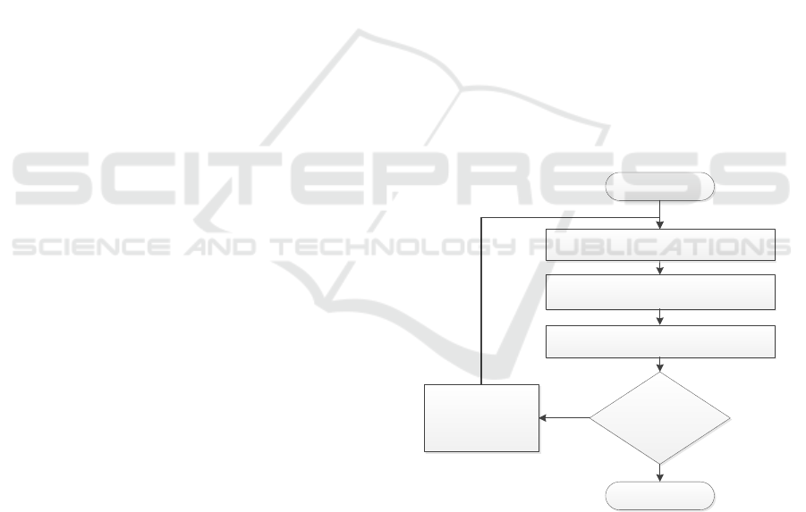
the training set (Figure 2). The successful

classification is considered as:

 Basic classification. Assignment of the pattern to

a cell representing only patterns of the same

category.

 Strict classification. Assignment of the pattern to

a cell according to the previous bullet and

additionally adjacent to only the same

(representing the same category) or empty cells

(not representing any pattern).

The selection of one of the above classification

methods is a parameter of the model.

Figure 2: Learning phase of the modified model (Vochozka

et al., 2017).

For the real use of the proposed model, two

criteria are crucial. The first one is the criterion of

learning termination in each step (level) of

hierarchical model learning. The criterion of the

maximum average shift distance between the 2D

layer cells defined in formula (4) was used.

The second criterion is that of the overall ability

of the whole set of learned sub-models to correctly

Training

set bigger then

limit?

Learn the model to the steady state

Store the learned model

Remove correctly

evaluated patterns

from training set

Initialize new Kohonen model

Start

Yes

Stop

Kohonen Map Modiﬁcation for Classiﬁcation Tasks

587

classify the training and later the test set of patterns

and can be implemented in several ways. The

minimum size of the training set, which still makes

sense for learning, was used in the model. Its higher

value reduces the number of hierarchical

classification steps but also limits the sensitivity of

the model.

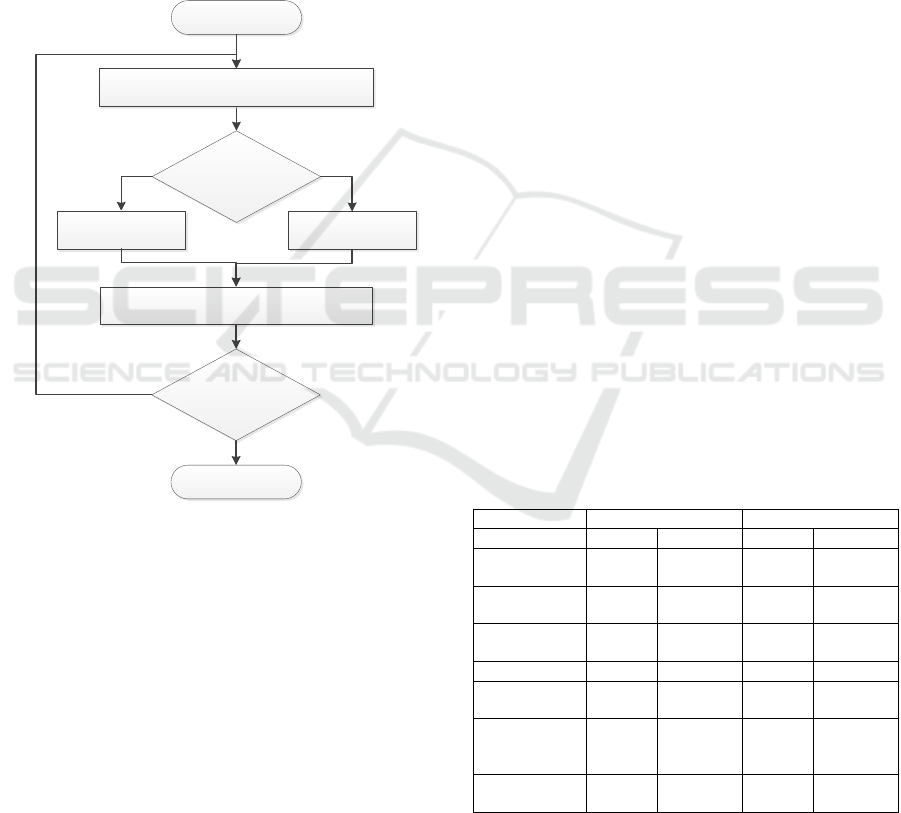
In the production phase (Figure 3), the

classification method differs depending on whether

we are in the last hierarchical step or not. For the last

model in the hierarchical structure, the probability

evaluation is always used, where the pattern is

assigned to the most likely category resulted from the

learning process.

Figure 3: Production phase of the modified model

(Vochozka et al., 2017).

The modified model was set up using 11

parameters including both the Kohonen map original

ones (used in each iteration) and the other ones

characterizing the hierarchical model's operation.

5 EXPERIMENTS

The experiments carried out were aimed at

confirming the preliminary hypothesis that both

modifications of the Kohonen map model are

beneficial to the generalization quality and hence the

classification of the test set of patterns. The first

group of experiments was focused on model behavior

with artificial data; the second group concentrated on

a comparison of results on standard datasets.

The first dataset was created to represent a

complex nonlinear transformation from the input

space R

to the space B

(Jelínek, 2018). 10,000

training and test patterns were generated with random

values of the coordinates from R

space uniformly

generated in the interval (0; 1).

One test set and two training sets were created.

From the training sets one was for the classical

learning of the model (only inputs from R

) and the

other one extended with the output b

(the network

input dimension increased to R

where the fifth

coordinate was b

). Experiments have been optimized

for maximizing the number of adequately classified

test patterns.

As mentioned above, the model has adjustable

parameters that significantly affect its results.

Manually searching for optimal setup would be

a lengthy process, and therefore, a superstructure of

the model was used implementing an optimization

mechanism based on genetic algorithms.

Two variants of the model’s setting have been

researched. The first one focused on modified model

learning and worked with a single level of the

hierarchical model (as if the model was not

hierarchically modified). The second variant also

involved a hierarchical modification of the model

structure, and the maximum number of levels was

limited to 10.

The best results are presented in the following

Table 1. These are the best from 406 experimental

settings of the model calculated by the genetic

algorithm for each variant.

Table 1: Best results for different settings (Jelínek, 2018).

Parameter

Max. 1 level

Max. 10 levels

Input

classic

extended

classic

extended

Number of

2D cells

40*40

35*35

40*40

35*35

Classification

criterion

basic

strict

Strict

Reduction

factor

0.2

0.3

Real levels

Total learning

iterations

118

238

515

Test patterns

correctly

classified

7998

8472

7985

8643

Model

success [%]

79.98

84.72

79.85

86.43

It is clear from the table that the use of the

modified learning process brings a significant

improvement in the classification capabilities of the

network over the original learning process. The key

Load next Kohonen model in the hierarchy

Start

Yes

Stop

Is it the

last model?

Use probability

based evaluation

Use absolute

evaluation

Evaluate all patterns in testing set

Was it the

last model?

Yes

ICAART 2019 - 11th International Conference on Agents and Artiﬁcial Intelligence

588

output is the finding that to achieve better results with

normalized data, the output values used for learning

(initially 0 and 1) must be reduced by the reduction

factor. Its appropriate setting was found by genetic

algorithm and was 0.2 or 0.3 (see the Reduction factor

row in Table 1).

The different number of 2D cells in different

scenarios also shows that model with extended input

set was able to obtain best results in the scenario with

fewer cells in the 2D layer, than the model with

standard input. The learning and overall performance

of the model with extended input were thus more

effective.

The sample visual outputs of the 2D network

shown in Figure 4 demonstrate the effect of modified

learning. The cells representing the patterns rated 0

are light grey, the patterns rated 1 are black. We get

"clean" colors for cells containing input patterns

included in only one category, for cells containing

patterns of different categories the color is mixed,

which respects the number of patterns in a cell with

different output categories. The influence of

additional output information on the final network

setting is quite apparent (right), and the fragmentation

from using the classical learning algorithm (left)

almost did not occur.

Figure 4: Influence of modified learning algorithm (Jelínek,

2018).

The results can still be improved by using

a hierarchical modification of the model; the added

value, however, is not so high in this case (quality

improvement of 1.71 %). The question, however, is

whether the appropriate data was used to maximize it.

In this case, the training set was evenly generated, but

the benefit could be more significant with data with

unequally represented output categories or different a

priori probabilities of them.

The second group of experiments was aimed at

comparing model results with other approaches on

standard datasets. They were obtained from the UCI

Machine Learning Repository (Dheeru and

Taniskidou, 2017). Three sets were selected with

different focus and number of input and output

attributes.

The first set is the Letter Recognition Data Set

(Lett) presented in (Frey and Slate, 1991). Input data

derive from black and white images of 26 alphabet

letters written in 20 different fonts; more images were

obtained by inserting random noise into existing ones.

Each input vector contains 16 values resulting from

the calculation of one-bit raster image values; the

output consists of a single value - the letter captured

on the figure. The set contains a total of 20 000

images. The rule-based classification method is also

presented in (Frey and Slate, 1991); the best rate of

correctly classified patterns is 82.7%.

To verify the presented model two disjoint sets

were created - for training (16000 patterns) and

testing (4000 patterns). The output was modified to

26 single-bit attributes (only one output value is one

for each letter, others are zero). Since the output is,

unlike the model description, not B

but B

, it was

necessary to select the winning attribute for the

output. The highest output attribute value does it.

Similar procedures also were used in the experiments

described below.

Experiments with this dataset did not reach the

expected values and did not achieve the reference

value mentioned in (Frey and Slate, 1991). The main

reason for this is difficult to identify, but it can be due

to the model parameter’s limits, especially in

conjunction with the R

> B

nonlinear

transformation. Inputs were pre-processed here,

which has reduced their number but has increased the

requirements on generalization capabilities of the

model too.

The second dataset was the Semeion Handwritten

Digit Data Set (Sem) described and used in

(Buscema, 1998). The set contains 1593 digital black

and white images in a 16x16 resolution. The output is

the only value identifying the digit. The article also

states the best classification using a combination of

several neural networks at 93.09%.

The input for our model was 256 binary attributes

(picture 16 x 16) and output ten binary values with the

same meaning as in the previous set and with the same

criterion for the best output selection. For the training

of the model, 1200 patterns were randomly selected,

for testing the remaining 393 ones (as recommended).

The results obtained with this dataset have already

met the expectations. The model was able to exceed

the reference value in the classification quality

(Buscema, 1998), and the influence of the extended

input data on the outputs of learning the model was

also positive.

The last used dataset was designed for testing of

accurate detection of room occupancy from data

obtained from several types of sensors. The set was

Kohonen Map Modiﬁcation for Classiﬁcation Tasks

589

published in (Candanedo and Feldheim, 2016) along

with an extensive set of experimental results. The data

are already divided into a training set of 8143 patterns

and two test sets (Occ 1 and Occ 2) of 2665 and 8926

patterns. The best-achieved classification results for

Occ 1 were 97.9% and for Occ 2 99.33%.

The original data were adapted for the use in our

experiment. The input was seven real normalized

values, and the output was one of two categories

(room occupied, empty).

The expected results were calculated for the

Occ 1 test set; the model again improved the best

result described in (Candanedo and Feldheim, 2016),

both for the classic and extended training set. For

Occ 2, however, the best classification was achieved

using standard input. This result has shown that the

model can achieve outstanding results even without

additional input information thanks to the hierarchical

structure of the model.

The worse outcome for the extended input can be

caused by the data character - fragmentation of

categories within the 2D layer was not significant,

and the model did not use this information. Instead, it

was forced to process more input data. Also, perhaps

a smaller size of the training set was not enough to

learn the given input-output transformation. The

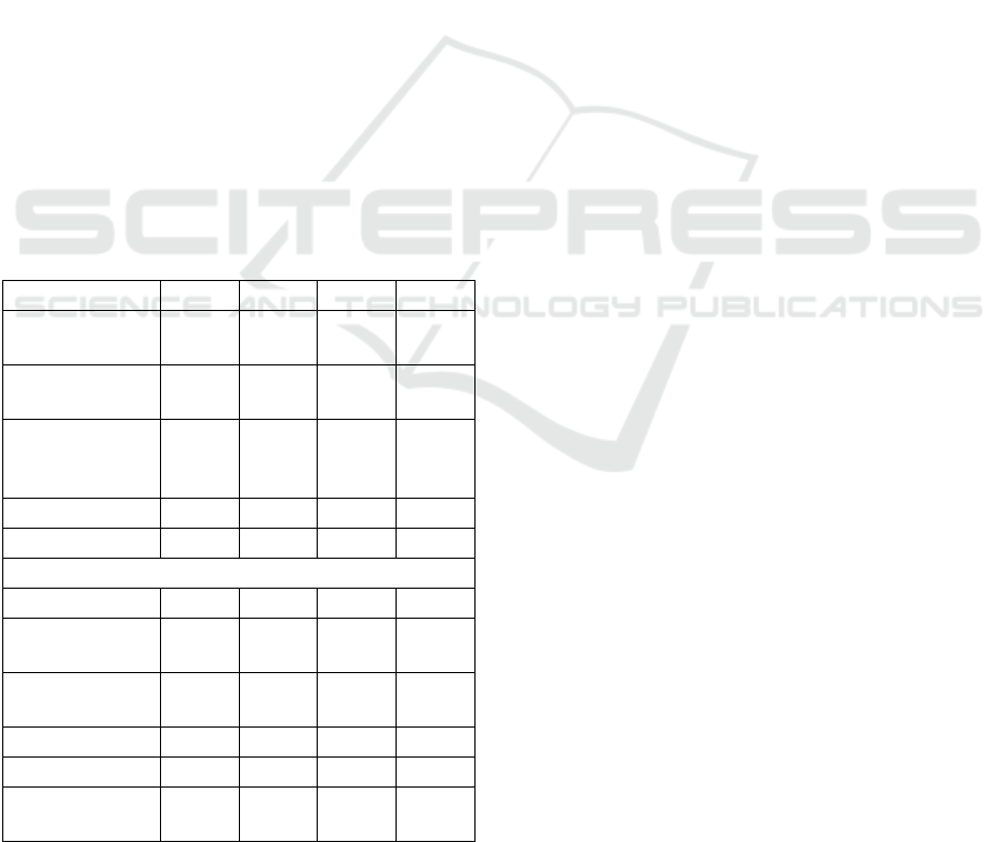
results of the experiments are summarized in Table 2.

Table 2: Results of experiments on standard datasets.

Data Set

Lett

Sem

Occ 1

Occ 2

Best reference

result [%]

82.7

93,1

97.9

99.3

Best result with

classic input [%]

42.0

94.7

99.6

99.9 *

Best result with

extended input

[%]

55.0 *

96.9 *

100.0 *

97.8

Training vectors

16000

1200

8143

Testing vectors

4000

393

2665

8926

Settings for best dataset result (*)

Input dimensions

256

Number of 2D

cells

20 * 20

40 * 40

10 * 10

20 *20

Classification

criterion

strict

Reduction factor

0.1

0.6

0.3

0.7

Real levels

Total learning

iterations

2723

186

2887

2399

6 CONCLUSIONS

This paper introduces a modified learning algorithm

for the Kohonen map, which enables solving of

classification tasks with this network. The core of the

modification is the use of an extended training set

using the output categorization of the training patterns

for the learning process. Modifications were made

even in setting the criteria for completing model

learning (criterion of minimal pattern shift in the 2D

layer). A visual superstructure of the model was

developed to allow a detailed study of the dynamics

of the model setup process, and the obtained

knowledge could be used to better understanding of

the learning process and the nature of input data.

The second significant modification is the design

and description of the behavior of a hierarchical

classification model based on modified Kohonen

maps. The training set is gradually reduced during the

process of learning, increasing the sensitivity of the

network to differences in input data. An algorithm for

the production phase of the model was developed,

based on the learned Kohonen map sub-models.

The model was described by a set of parameters,

whose values had to be empirically determined.

Therefore, genetic algorithms have been used to find

optimal values.

Two groups of experiments were carried out with

the modified model. Experiments on artificial dataset

were focused on model in-depth behavior to verify

the benefits of the proposed modifications. They

confirmed the positive influence of the training set

extended by the outputs and the hierarchical structure

of the model for better performance of the

classification model. The overall classification

quality was improved by 6.58% on the generated data

with nonlinear randomly selected transformation

function R

> B

. The benefit of the hierarchical

structure would probably be higher when using data

unevenly covering the input space.

The experiments on standard datasets were used

to obtain result comparable with other research and to

show the practical usability of the model. Three

datasets were used in four experiments. In three of

them, the presented model exceeded the best

classification quality mentioned in the references.

Although the described model gives better results

with unprocessed data than literature references, there

is still the space for improvement of its concept. We

can find open questions in the definition and possible

dynamic modification of the neighborhood of the

winning cell, the type of distance calculation used in

the 2D layer, or the criteria for completing the

individual steps of the hierarchical learning process.

ICAART 2019 - 11th International Conference on Agents and Artiﬁcial Intelligence

590

It will also be necessary to examine the impact of the

input data structure on the results achieved.

REFERENCES

Buscema, M., 1998. Metanet*: The theory of independent

judges. Substance use & misuse, 33(2), 439-461.

Candanedo, L. M. and Feldheim, V., 2016. Accurate

occupancy detection of an office room from light,

temperature, humidity and CO2 measurements using

statistical learning models. Energy and Buildings, 112,

28-39.

Carpenter, G. A. and Grossberg, S., 1987. ART 2: Self-

organization of stable category recognition codes for

analog input patterns. In Applied optics, Vol. 26(23),

pp. 4919-4930.

Dheeru, D. and Taniskidou, E. K., 2017. UCI machine

learning repository. University of California, Irvine,

School of Information and Computer Sciences.

Frey, P. W. and Slate, D. J., 1991. Letter Recognition Using

Holland-style Adaptive Classifiers. In Machine

Learning, Vol 6 #2 March 91.

Fritzke, B., 1994. Growing cell structures—a self-

organizing network for unsupervised and supervised

learning. Neural networks, 7(9), 1441-1460.

Jelínek, J., 1992. Exceptional working states of power

grids. CTU - FEE, Prague. (in Czech).

Jelínek, J., 2018. Classification Model Based on Kohonen

Maps. In Proceedings of the Conference ACIT 2018,

Ternopil National Economic University, pp. 145-148.

Kohonen, T., 1982. Self-organized formation of

topologically correct feature maps. In Biological

cybernetics, Vol. 43(1), pp. 59-69.

McCulloch, W., S. and Pitts, W., 1943. A logical calculus

of the ideas immanent in nervous activity. In The

Bulletin of mathematical biophysics, Vol. 5(4), pp. 115-

133.

Rauber, A., Merkl, D. and Dittenbach, M., 2002. The

growing hierarchical self-organizing map: exploratory

analysis of high-dimensional data. IEEE Transactions

on Neural Networks, 13(6), 1331-1341.

Rosenblatt, F., 1957. The perceptron, a perceiving and

recognizing automaton Project Para. Cornell

Aeronautical Laboratory.

Rumelhart, D., E., Hinton, G., E. and Williams, R., J., 1986.

Learning representations by back-propagating errors. In

Nature, Vol. 323.9.

Vochozka, M., Jelínek, J., Váchal, J., Straková, J. and

Stehel, V., 2017. Using neural networks for

comprehensive business evaluation. H. C. Beck,

Prague, ISBN 978-80-7400-642-5 (in Czech).

Kohonen Map Modiﬁcation for Classiﬁcation Tasks

591