Makespan Minimization with Sequence-dependent
Non-overlapping Setups
Marek Vlk
1,2
, Antonin Novak
2,3
and Zdenek Hanzalek
2
1
Department of Theoretical Computer Science and Mathematical Logic, Faculty of Mathematics and Physics,
Charles University, Czech Republic
2
Industrial Informatics Department, Czech Institute of Informatics, Robotics, and Cybernetics,
Czech Technical University in Prague, Czech Republic
3
Department of Control Engineering, Faculty of Electrical Engineering,
Czech Technical University in Prague, Czech Republic
Keywords:
Human Resource Scheduling, Common Setup Operator, Constraint Programming, Hybrid Heuristic.
Abstract:
This paper deals with a scheduling problem that emerges in the production of water tubes of different sizes
that require reconfiguration of the machines. The reconfiguration of the machines leads to the notion of
sequence-dependent setup times between tasks. These setups are often performed by a single person who
cannot serve more than one machine at the same moment, i.e., the setups must not overlap. Surprisingly, the
problem with non-overlapping setups has received only a little attention so far. To solve this problem, we
propose an Integer Linear Programming formulation, Constraint Programming models and a hybrid heuristic
that leverages the strength of Integer Linear Programming in the shortest Hamiltonian path problem and the
efficiency of Constraint Programming at sequencing problems with makespan minimization. The experimental
evaluation shows that among the proposed exact approaches, the Constraint Programming is a superior method
being able to solve instances with 3 machines and up to 11 tasks on each machine to optimality within a few
seconds. The proposed hybrid heuristic attains high-quality solutions for instances with 50 machines and up
to 116 tasks on each machine.
1 INTRODUCTION
The problem studied in this paper is inspired by a con-
tinuous production of plastic water tubes. In such pro-
ductions, the factory brings in the material in form
of plastic granulate that is being in-house processed.
The manufacturer has a stack of orders for manufac-
turing plastic tubes of various widths and lengths. The
production has 13 machines that can produce differ-
ent tubes in parallel. Different variants of tubes re-
quire different settings of the machines. Hence, when
switching from one type of tube to another, a machine
setter is required to visit the particular machine and
make the tool adjustment. The goal is to process all
orders as fast as possible.
As the tool adjustment is done by a single machine
setter, he or she is likely to be the bottleneck of the
production when the orders are not scheduled well.
Given the assignment of the orders to the machines,
the basic idea is to cluster similar tube variants next
to each other, as these require little or no setup time
to adjust the tool.
We model the problem as a scheduling problem
where the tasks are dedicated to the machines and
have sequence-dependent setup times. Each setup oc-
cupies an extra resource that is assumed to be unary,
hence setups must not overlap in time. The goal is
to minimize the makespan of the overall schedule. In
this paper, we design an Integer Linear Programming
(ILP) model, three variants of Constraint Program-
ming (CP) model, and a heuristic algorithm.
The main contributions of this paper are:
• formal definition of a new problem with non-
overlapping setups
• exact approaches based on ILP and CP for-
malisms
• a very efficient hybrid heuristic yielding optimal
or near-optimal schedules
The rest of the paper is organized as follows. We
first survey briefly the existing work in the related
area. Next, Section 3 gives the formal definition of
the problem at hand. In Section 4, we describe an
ILP model, while in Section 5 we introduce three
Vlk, M., Novak, A. and Hanzalek, Z.
Makespan Minimization with Sequence-dependent Non-overlapping Setups.
DOI: 10.5220/0007362700910101
In Proceedings of the 8th International Conference on Operations Research and Enterprise Systems (ICORES 2019), pages 91-101
ISBN: 978-989-758-352-0
Copyright
c
 2019 by SCITEPRESS – Science and Technology Publications, Lda. All rights reserved
91

c
max
c
max
tt
o
1,2,3
o
1,2,3
o
1,2,3
o
1,2,3
o
2,1,3
o
2,1,3
o
2,2,1
o
2,2,1
o
2,1,3
o
2,1,3
o
2,2,1
o
2,2,1
o
1,1,2
o
1,1,2
o
3,3,2
o
3,3,2
o
3,2,1
o
3,2,1
o
3,3,2
o
3,3,2
o
3,2,1
o
3,2,1
o
1,1,2
o
1,1,2
M
1
M
1
M
2
M
2
M
3
M
3
T
1,1
T
1,1
T
1,2
T
1,2
T
2,1
T
2,1
T
2,2
T
2,2
T
1,3
T
1,3
T
2,3
T
2,3
T
3,2
T
3,2
T
3,3
T
3,3
T
3,1
T
3,1
HH
(a) Feasible schedule.
c
max
c
max
tt
M
1
M
1
M
2
M
2
M
3
M
3
T
1,1
T
1,1
T
1,2
T
1,2
T
1,3
T
1,3
T
2,1
T
2,1
T
2,2
T
2,2
T
2,3
T
2,3
T
3,1
T
3,1
T
3,2
T
3,2
T
3,3
T
3,3
HH
(b) Infeasible schedule, setups are overlapping.
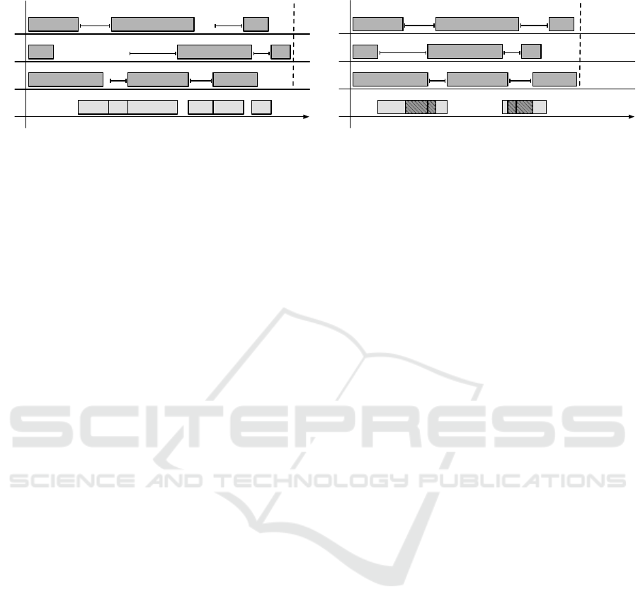
Figure 1: An illustration of a schedule with three machines and three tasks to be processed on each machine.
variants of a CP model, and in Section 6 we propose
the heuristic algorithm. Finally, we present computa-
tional experiments in Section 7 and draw conclusions
in Section 8.
2 RELATED WORK
There is a myriad of papers on scheduling with
sequence-dependent setup times or costs (Allahverdi
et al., 2008), proposing exact approaches (Lee and
Pinedo, 1997) as well as various heuristics (Vallada
and Ruiz, 2011). But the research on the problems
where the setups require extra resource is scarce.
An unrelated parallel machine problem with ma-
chine and job sequence-dependent setup times, stud-
ied by (Ruiz and Andr
´
es-Romano, 2011), considers
also the non-renewable resources that are assigned to
each setup, which affects the amount of time the setup
needs and which is also included in the objective func-
tion. On the other hand, how many setups may be
performed at the same time is disregarded. The au-
thors propose a Mixed Integer Programming formula-
tion along with some static and dynamic dispatching
heuristics.
A lotsizing and scheduling problem with a com-
mon setup operator is tackled in (Tempelmeier and
Buschk
¨
uhl, 2008). The authors give ILP formula-
tions for what they refer to as a dynamic capacitated
multi-item multi-machine one-setup-operator lotsiz-
ing problem. Indeed, the setups to be performed by
the setup operator are considered to be scheduled such
that they do not overlap. However, these setups are
not sequence-dependent in the usual sense. The se-
tups are associated to a product whose production is
to be commenced right after the setup and thus the
setup time, i.e., the processing time of the setup, does
not depend on a pair of tasks but only on the succeed-
ing task.
A complex problem that involves machines requir-
ing setups that are to be performed by operators of dif-
ferent capabilities has been addressed in (Chen et al.,
2003). The authors modeled the whole problem in
the time-indexed formulation and solved it by decom-
posing the problem into smaller subproblems using
Lagrangian Relaxation and solving the subproblems
using dynamic programming. A feasible solution is
then composed of the solutions to the subproblems by
heuristics, and, if impossible, the Lagrangian multi-
pliers are updated using surrogate subgradient method
as in (Zhao et al., 1999). The down side of this ap-
proach is that the time-indexed formulation yields a
model of pseudo-polynomial size. This is not suitable
for our problem as it poses large processing and setup
times.
To the best of our knowledge, this is the first pa-
per that efficiently solves the scheduling problem with
dedicated machines with sequence-dependent non-
overlapping setups.
3 PROBLEM STATEMENT
Informally speaking, the problem tackled in this pa-
per consists of a set of machines and a set of indepen-
dent non-preemptive tasks, each of which is dedicated
to one particular machine where it will be processed.
Also, there are sequence-dependent setup times on
each machine. In addition, these setups are to be per-
formed by a human operator who is referred to as a
machine setter. Such a machine setter cannot per-
form two or more setups at the same time. It follows
that the setups on all the machines must not over-
lap in time. Examples of a feasible and an infeasi-
ble schedule with 3 machines can be seen in Fig. 1.
Even though the schedule (Fig. 1b) on the machines
contains setup times, such schedule is infeasible since
it would require overlaps in the schedule for the ma-
chine setter.
The aim is to find a schedule that minimizes the
completion time of the latest task. It is clear that the
latest task is on some machine and not in the sched-
ICORES 2019 - 8th International Conference on Operations Research and Enterprise Systems
92

ule of a machine setter since the completion time of
the last setup is followed by at least one task on a ma-
chine.
3.1 Formal Definition
Let M = {M
1
,...,M
m
} be a set of machines and for
each M
i
∈ M, let T
(i)
= {T
i,1
,..., T
i,n
i
} be a set of
tasks that are to be processed on machine M
i
, and let
T =
S
M
i
∈M
T
(i)
= {T
1,1
,..., T
m,n
m
} denote the set of all
tasks. Each task T
i, j
∈ T is specified by its processing
time p
i, j
∈ N. Let s
i, j
∈ N
0
and C
i, j
∈ N be start time
and completion time, respectively, of task T
i, j
∈ T ,
which are to be found. All tasks are non-preemptive,
hence, s
i, j
+ p
i, j
= C
i, j
must hold.
Each machine M
i
∈ M performs one task at a time.
Moreover, the setup times between two consecutive
tasks processed on machine M
i
∈ M are given in ma-
trix O
(i)
∈ N
n
i
×n
i
. That is, o
i, j, j
0
= (O
(i)
)
j, j
0
deter-
mines the minimal time distance between the start
time of task T
i, j
0
and the completion time of task T
i, j
if
task T
i, j
0
is to be processed on machine M
i
right after
task T
i, j
, i.e., s
i, j
0
−C
i, j
≥ o
i, j, j
0
must hold.
Let H = {h
1
,. .. ,h
`
}, where ` =
∑
M
i
∈M
n
i
− 1, be
a set of setups that are to be performed by the machine
setter. Each h
k
∈ H corresponds to the setup of a pair
of tasks that are scheduled to be processed in a row on
some machine. Thus, function st : H −→ M × T × T is
to be found. Also, s
k
∈ N
0
and C
k
∈ N are start time
and completion time of setup h
k
∈ H, which are to
be found. Assuming h
k
∈ H corresponds to the setup
between tasks T
i, j
∈ T and T
i, j
0
∈ T , i.e., st(h
k
) =
(M
i
,T
i, j
,T
i, j
0
), it must hold that s
k
+ o
i, j, j
0
= C
k
, also
C
i, j
≤ s
k
, and C
k
≤ s
i, j
0
. Finally, since the machine set-
ter may perform at most one task at any time, it must
hold that, for each h
k
,h
k
0
∈ H,k 6= k
0
, either C
k
≤ s
k
0
or C
k
0
≤ s
k
.
The objective is to find such a schedule that min-
imizes the makespan, i.e., the latest completion time
of any task:
min max
T
i, j
∈T
C
i, j
(1)
It is easy to see that such problem is strongly
N P -hard even for the case of one machine, i.e.,
m = 1, which can be shown by the reduction from
the shortest Hamiltonian path problem.
In the following sections, we propose two exact
approaches.
4 INTEGER LINEAR
PROGRAMMING MODEL
The proposed formulation models the problem with
two parts. The first part handles scheduling of tasks
on the machines using efficient rank-based model
(Lasserre and Queyranne, 1992). This approach uses
binary variables x
i, j,q
to encode whether task T
i, j
∈
T
(i)
is scheduled on q-th position in the permutation
on machine M
i
∈ M. Another variable is τ
i,q
denot-
ing the start time of a task that is scheduled on q-th
position in the permutation on machine M
i
∈ M.
The second part of the model resolves the ques-
tion, in which order and when the setups are per-
formed by a machine setter. There, we need to sched-
ule all setups H, where the setup time π
k
of the setup
h
k
∈ H is given by the corresponding pair of tasks on
the machine.
Let us denote the set of all natural numbers up to n
as [n] = {1,. ..,n}. We define the following function
φ : H → M ×[max
M
i
∈M
n
i
] (e.g., φ(h
k
) = (M
i
,q)), that
maps h
k
∈ H to setups between the tasks scheduled at
positions q and q + 1 on machine M
i
∈ M. Since the
time of such setup is a variable (i.e., it depends on the
pair of consecutive tasks on M
i
), rank-based model
would not be linear. Therefore, we use the relative-
order (also known as disjunctive) model (Applegate
and Cook, 1991; Balas, 1968) that admits processing
time given as a variable. Its disadvantage over the
rank-based model is that it introduces a big M con-
stant in the constraints, whereas the rank-based model
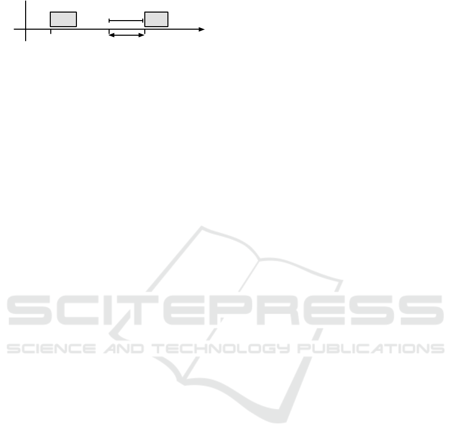
does not. See Fig. 2 for meaning of the variables.
The full model is stated as:
min C
max
(2)
s.t.
C
max
≥ τ
i,n
i
+
∑
T
i, j
∈T
(i)
p
i, j
· x
i, j,n
i
∀M
i
∈ M (3)
∑
q∈[n
i
]
x
i, j,q
= 1 ∀M
i
∈ M,∀T
i, j
∈ T
(i)
(4)
∑
T
i, j
∈T
(i)
x
i, j,q
= 1 ∀M
i
∈ M,∀q ∈ [n
i
] (5)
s
k
+ π
k
≤ s
l
+ M · (1 − z
k,l
) (6)
∀h
l
,h
k
∈ H : l < k
s
l
+ π
l
≤ s
k
+ M · z
k,l
∀h
l
,h
k
∈ H : l < k (7)
π
k
≥ o
i, j, j
0
· (x
i, j,q
+ x
i, j
0
,q+1
− 1) (8)
∀h
k
∈ H : φ(h
k
) = (M
i
,q), ∀T
i, j
,T
i, j
0
∈ T
(i)
s
k
+ π
k
≤ τ
i,q+1
(9)
∀h
k
∈ H : φ(h
k
) = (M
i
,q)
s
k
≥ τ
i,q
+
∑
T
i, j
∈T
(i)
p
i, j
· x
i, j,q
(10)
Makespan Minimization with Sequence-dependent Non-overlapping Setups
93

M
i
M
i
qq
q +1q +1
h
k
h
k
⌧
i,q
⌧
i,q
⌧
i,q+1
⌧
i,q+1
s
k
s
k
⇡
k
⇡
k
tt
Figure 2: Meaning of the variables in the model.
∀h
k
∈ H : φ(h
k
) = (M
i
,q)
where
C
max
∈ R
+
0
(11)
τ
i,q
∈ R
+
0
∀M
i
∈ M,∀q ∈ [n
i
] (12)
s
k
,π
k
∈ R
+
0
∀h
k
∈ H (13)
x
i, j,q
∈ {0, 1} (14)
∀M
i
∈ M,∀T
i, j
∈ T
(i)
,∀q ∈ [n
i
]
z
k,l
∈ {0, 1} ∀h
k
,h
l
∈ H : l < k (15)
The constraint (3) computes makespan of the sched-
ule while constraints (4)–(5) states that each task oc-
cupies exactly one position in the permutation and
that each position is occupied by exactly one task.
Constraints (6) and (7) guarantee that setups do not
overlap. M is a constant that can be set as |H| ·
max
i
O
(i)
. Constraint (8) sets processing time π
k
of
the setup h
k
∈ H to o
i, j, j
0
if task T
i, j
0
is scheduled on
machine M
i
right after task T
i, j
. Constraints (9) and
(10) are used to avoid conflicts on machines. The con-
straint (9) states that a task cannot start earlier than
its preceding setup finishes. Similarly, the constraint
(10) states that a setup is scheduled after the corre-
sponding task on the machine finishes.
4.1 Formulation for a Single Machine
The problem with a single machine (M
i
∈ M) reduces
to the shortest Hamiltonian path in the graph defined
by setup time matrix O
(i)
. To solve this problem, we
transform it to the Traveling Salesperson Problem by
introducing a dummy task T
i,0
∈ T
(i)0
= T
(i)
∪ {T
i,0
}
that has zero setup times with all other tasks, i.e.,
o
i,0, j
= o
i, j,0
= 0, ∀T
i, j
∈ T
(i)0
. Then, we use a well-
known sub-tour elimination (Applegate et al., 2011;
Pferschy and Stan
ˇ
ek, 2017) ILP model to solve it:
min
∑
T
i, j
∈T
(i)0
∑
T
i, j
0
∈T
(i)0
o
i, j, j
0
· y
j, j
0
+
∑
T
i, j
∈T
(i)0
p
i, j
(16)
s.t.
∑
T
i, j
∈T
(i)0
y
j, j
0
= 1 ∀T
i, j
0
∈ T
(i)0
(17)
∑
T
i, j
0
∈T
(i)0
y
j, j
0
= 1 ∀T
i, j
∈ T
(i)0
(18)
∑
T
i, j
,T
i, j
0
∈S
y
j, j
0
≤ |S| − 1 ∀S ⊂ T
(i)0
(19)
where
y
j, j
0
∈ {0, 1} ∀T
i, j
,T
i, j
0
∈ T
(i)0
(20)
The variable y
j, j
0
indicates whether task T
i, j
is imme-
diately followed by task T
i, j
0
. We solve the model in a
lazy way, i.e., without constraints (19), that are lazily
generated during the solution by a depth-first search
algorithm. Note that the machine setter does not need
to be modeled for the single machine problem.
4.2 Additional Improvements
We use the following improvements of the model that
have a positive effect on the solver performance.
1. Warm Starts. The solver is supplied with an ini-
tial solution. It solves a relaxed problem, where it
relaxes on the condition that setups do not over-
lap. Such solution is obtained by solving the
shortest Hamiltonian path problem given by setup
time matrix O
(i)
independently for each machine
M
i
∈ M, as described in Section 4.1. Since such
solution might be infeasible for the original prob-
lem, we transform it in a polynomial time into a
feasible one. It is done in the following way. For
each setup among all machines, we set the start
time of k-th setup on machine M
i
, i ≥ 2, to the
completion time of k-th setup on machine M
i−1
.
For the setups on machine M
1
, the start time of
(k + 1)-th setup is set to the completion time of
k-th setup on machine M
m
.
2. Lower Bounds. We supply a lower bound on
C
max
variable given as the maximum of all best
proven lower bounds of model (16)–(20) among
all machines M
i
∈ M (see Section 4.1).
3. Pruning of Variables. We can reduce the number
of variables in the model due to the structure of the
problem. We fix values of some of the z
k,l
vari-
ables according to the following rule. Let h
k
,h
l
∈
H such that φ(h
k
) = (M
i
,q) and φ(h
l
) = (M
i
,v)
for any M
i
∈ M. Then, q < v ⇒ z
k,l
= 1 holds in
some optimal solution. Note that the rule holds
only for setups following from the same machine.
The rule states that the relative order of setups on
the same machine is determined by the natural or-
dering of task positions on that machine. See for
example setups o
1,1,2
and o
1,2,3
in Fig. 1. Since
these setups follow from the same machine, their
relative order is already predetermined by posi-
tions of the respective tasks. We note that the pre-
solve of the solver was not able to deduce these
rules on its own.
ICORES 2019 - 8th International Conference on Operations Research and Enterprise Systems
94

5 CONSTRAINT
PROGRAMMING MODELS
Another way how the problem at hand can be tack-
led is to use the modeling approach based on the
Constraint Programming (CP) formalism, where spe-
cial global constraints modeling unary (disjunctive)
resources and efficient filtering algorithms are used
(Vil
´
ım et al., 2005). These concepts work with inter-
val variables whose start time and completion time
are denoted by predicates StartO f and EndO f , and
the difference between the completion time and the
start time of the interval variable can be set using
predicate LengthO f .
The CP models are constructed as follows. We
introduce interval variables I
i, j
for each T
i, j
∈ T , and
the lengths of these interval variables are set to the
corresponding processing times:
LengthO f (I
i, j
) = p
i, j
(21)
The sequence is resolved using the NoOverlap
constraint. The NoOverlap(I) constraint on a set I of
interval variables states that it constitutes a chain of
non-overlapping interval variables, any interval vari-
able in the chain being constrained to be completed
before the start of the next interval variable in the
chain. In addition, the NoOverlap(I, O
(i)
) constraint
is given a so-called transition distance matrix O
(i)
,
which expresses a minimal delay that must elapse be-
tween two successive interval variables. More pre-
cisely, if I
i, j
,I
i, j
0
∈ I, then (O
(i)
)
j, j
0
gives a minimal
allowed time difference between StartO f (I
j
0
) and
EndO f (I
j
). Hence, the following constraint is im-
posed, ∀M
i
∈ M:
NoOverlap

[
T
i, j
∈T
(i)
{I
i, j
} , O
(i)

(22)
The objective function is to minimize the
makespan:
min max
T
i, j
∈T
EndO f (I
i, j
) (23)
This model would already solve the problem if the
setups were not required to be non-overlapping. In
what follows we describe three ways how the non-
overlapping setups are resolved. Constraints (21)–
(23) are part of each of the following model.
5.1 CP1: with Implications
Let us introduce I
st
i, j
for each T
i, j
∈ T representing the
setup after task T
i, j
. There is
∑
M
i
∈M
n
i
such variables.
To ensure that the setups do not overlap in time is en-
forced through the following constraint:
NoOverlap

[
T
i, j
∈T
{I
st
i, j
}

(24)
Notice that this constraint is only one and it is over
all the interval variables representing setups on all
machines. This NoOverlap constraint does not need
any transition distance matrix as the default values 0
are desired.
Since it is not known a priori which task will be
following task T
i, j
, the quadratic number of implica-
tions determining the precedences and lengths of the
setups must be imposed. For this purpose, the predi-
cate Next is used. Next(I) equals the interval variable
that is to be processed in the chain right after interval
variable I. Thus, the following constraints are added,
∀M
i
∈ M,∀T
i, j
,T
i, j
0
∈ T
(i)
, j 6= j
0
:
Next(I
i, j
) = I
i, j
0
⇒ EndO f (I
i, j
) ≤ StartO f (I
st
i, j
) (25)
Next(I
i, j
) = I
i, j
0
⇒ EndO f (I
st
i, j
) ≤ StartO f (I
i, j
0
) (26)
Next(I
i, j
) = I
i, j
0
⇒ LengthO f (I
st
i, j
) = o
i, j, j
0
(27)
Note that the special value when an interval vari-
able is the last one in the chain is used to turn the last
setup on a machine into a dummy one.
5.2 CP2: with Element Constraints
We did not find a way how to avoid the quadratic num-
ber of implications for setting the precedences, but at
least setting the lengths of the setups can be substi-
tuted by the element constraint, which might be bene-
ficial as global constraints are usually more efficient.
More precisely, this model contains also constraints
(24), (25), and (26), but constraint (27) is substituted
as follows.
Assume the construct Element(Ar ray, k) returns
the k-th element of Array, (O
(i)
)
j
is the j-th row of
matrix O
(i)
, and IndexO f Next(I
i, j
) returns the index
of the interval variable that is to be processed right
after I
i, j
. Then the following constraint is added, for
each I
st
i, j
:
LengthO f (I
st
i, j
) = Element

(O
(i)
)
j
, IndexO f Next(I
i, j
)

(28)
5.3 CP3: with Optional Interval
Variables
In this model, we use the concept of optional interval
variables (Laborie et al., 2009). An optional inter-
val variable can be set to be present or absent. The
Makespan Minimization with Sequence-dependent Non-overlapping Setups
95

predicate PresenceO f is used to determine whether
or not the interval variable is present in the resulting
schedule. Whenever an optional interval variable is
absent, all the constraints that are associated with that
optional interval variable are implicitly satisfied and
predicates StartO f , EndO f , and LengthO f are set to
0.
Hence, we introduce optional interval variable
I
opt
i, j, j
0
for each pair of distinct tasks on the same ma-
chine, i.e., ∀M
i
∈ M,∀T
i, j
,T
i, j
0
∈ T
(i)
, j 6= j
0
. There
are
∑
M
i
∈M
n
i
(n
i
− 1) such variables. The lengths of
these interval variables are set to corresponding setup
times:
LengthO f (I
opt
i, j, j
0
) = o
i, j, j
0
(29)
To ensure that the machine setter does not perform
more than one task at the same time, the following
constraint is added:
NoOverlap

[
T
i, j
,T
i, j
0
∈T
j6= j
0
{I
opt
i, j, j
0
}

(30)
In this case, to ensure that the setups are indeed
processed in between two consecutive tasks, we use
the constraint EndBe f oreStart(I
1
,I
2
), which ensures
that interval variable I
1
is completed before interval
variable I
2
can start, but if either of the interval vari-
ables is absent, the constraint is implicitly satisfied.
Thus, the following constraints are added, ∀I
opt
i, j, j
0
:
EndBe f oreStart(I
i, j
,I
opt
i, j, j
0
) (31)
EndBe f oreStart(I
opt
i, j, j
0
,I
i, j
0
) (32)
Finally, in order to ensure the correct presence of
optional interval variables, the predicate PresenceO f
is used. Thus, the following constraint is imposed,
∀I
opt
i, j, j
0
:
PresenceO f (I
opt
i, j, j
0
) ⇔ Next(I
i, j
) = I
i, j
0
(33)
5.4 Additional Improvements
We use the following improvements:
1. Search Phases. Automatic search in the solver is
well tuned-up for most types of problems, lever-
aging the newest knowledge pertaining to variable
selection and value ordering heuristics. In our
case, however, preliminary results showed that the
solver struggles to find any feasible solution al-
ready for small instances. It is clear that it is
easy to find some feasible solution, e.g., by set-
ting an arbitrary order of tasks on machines and
then shifting the tasks to the right such that the
setups do not overlap. To make the solver find
always some feasible solution at a blow, we set
the search phases such that the sequences on ma-
chines are resolved first, and then the sequences
of setups for the machine setter are resolved. This
is included in all the CP models described.
2. Warm Starts. Similarly to improvement (1) in
Section 4.2, we boost the performance by provid-
ing the solver with a starting point. We do this
only for CP3 as the preliminary numerical exper-
iments showed a slight superiority of CP3.
More precisely, we first find an optimal sequence
of tasks minimizing makespan on each machine
separately, as described in Section 4.1, and then
we set those interval variables I
opt
i, j, j
0
to be present
if T
i, j
0
is sequenced directly after T
i, j
on machine
M
i
. This is all that we set as the starting point. No-
tice that unlike in Section 4.2, we do not calculate
the complete solution but we let the solver do it.
The solver then quickly completes the assignment
of all the variables such that it gets a solution of
reasonably good objective value.
Note that the optimal sequences on machines are
solved using ILP so it can be seen as a hybrid ap-
proach. This model with warm starts is in what
follows referred to as CP3ws.
6 HEURISTIC APPROACH
We propose an approach that guides the solver
quickly towards solutions of very good quality but
cannot guarantee optimality of what is found. There
are two main phases of this approach. In the first
phase, the model is decomposed such that its subprob-
lems are solved optimally or near-optimally and then
the solutions of the subproblems are put together so
as to make a correct solution of the whole problem.
In the second phase, the solution found is locally im-
proved by repeatedly adjusting the solution in promis-
ing areas. More details follow.
6.1 Decomposition Phase
The idea of the model decomposition is as follows.
First, again, we find an optimal sequence of tasks
minimizing makespan on each machine separately,
as described in Section 4.1. Second, given these se-
quences on each machine, the setups to be performed
are known, hence, the lengths of the setups are fixed
as well as the precedence constraints with respect to
ICORES 2019 - 8th International Conference on Operations Research and Enterprise Systems
96

11
dd
dd
dd
dd
11
M
1
M
1
M
2
M
2
3d +13d +1
tt
HH
(a) A problem instance where optimal sequences on ma-
chines lead to a sub-optimal solution.
dd
dd
11
d +1d +1
11
dd
2d +32d +3
M
1
M
1
M
2
M
2
tt
HH
(b) Sub-optimal sequence on one machine yields a glob-
ally optimal solution.
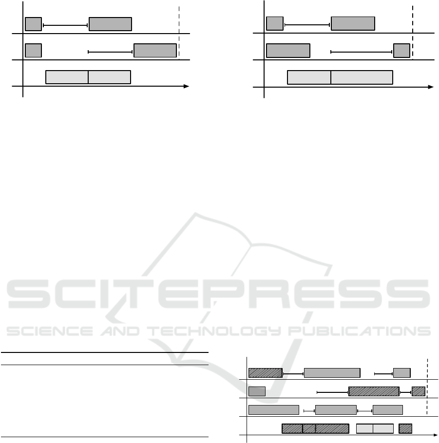
Figure 3: Solving the problem greedily for each machine separately can lead to arbitrarily bad solutions. The numbers depict
the processing times of the tasks and setups.
the tasks on machines. Thus, all that needs to be re-
solved is the order of setups.
The pseudocode is given in Algorithm 1. It takes
one machine at a time and finds an optimal sequence
for it while minimizing makespan. The time limit
for the computation of one sequence on a machine
is given in such a way that there is a proportional re-
maining time limit for the rest of the algorithm. OP-
TIMALSEQ(i, TimeLimit) returns the best sequence
it finds on machine M
i
∈ M in the given TimeLimit.
The TimeLimit is computed using RemainingTime(),
which is the time limit for the entire run of the algo-
rithm minus the time that already elapsed from the be-
ginning of the run of the algorithm. In the end, the so-
lution is found using the knowledge of the sequences
on each machine M
i
∈ M.
Algorithm 1: Solving the decomposed model.
function SOLVEDECOMPOSED
for each M
i
∈ M do
TimeLimit ← RemainingTime()/(m − i + 2)
Seq
i
← OPTIMALSEQ(i, TimeLimit)
end for
Return SOLVE(Seq, RemainingTime())
end function
Clearly, this decomposition may lead to a schedule
arbitrarily far from the optimum. Consider a problem
depicted in Fig. 3. It consists of two machines, M
1
and M
2
, and two tasks on each machine, with pro-
cessing times p
1,1
= p
2,1
= 1, p
1,2
= p
2,2
= d, where
d is any constant greater than 2, and with setup times
o
1,1,2
= o
2,1,2
= d,o
1,2,1
= o
2,2,1
= d + 1. Then, op-
timal sequence on each machine yields a solution of
makespan 3d + 1, whereas choosing sub-optimal se-
quence on either of the machines gives optimal objec-
tive value 2d + 3.
6.2 Improving Phase
Once we have some solution to the problem, the
idea of the heuristic is to improve it applying
the techniques known as local search (Hentenryck
and Michel, 2009) and large neighborhood search
(Pisinger and Ropke, 2010).
It is clear that in order to improve the solution,
something needs to be changed on the critical path,
which is such a sequence of setups and tasks on ma-
chines that the completion time of the last task equals
the makespan and that none of these tasks and setups
can be shifted to the left without violating resource
constraints (see an example in Fig. 4). Hence, we find
the critical path first.
c
max
c
max
tt
o
1,2,3
o
1,2,3
o
1,2,3
o
1,2,3
o
2,2,1
o
2,2,1
o
2,1,3
o
2,1,3
o
1,1,2
o
1,1,2
o
3,3,2
o
3,3,2
o
3,2,1
o
3,2,1
o
3,2,1
o
3,2,1
M
1
M
1
M
2
M
2
M
3
M
3
T
1,2
T
1,2
T
2,2
T
2,2
T
1,3
T
1,3
T
3,2
T
3,2
T
3,3
T
3,3
T
3,1
T
3,1
HH
Figure 4: An illustration of the critical path depicted by
dashed rectangles.
The most promising place to be changed on the
critical path could be the longest setup. Hence, we
find the longest setup on the critical path, then we
prohibit the two consecutive tasks corresponding to
the setup from being processed in a row again and
re-optimize the sequence on the machine in question.
Two tasks are precluded from following one another
by setting the corresponding setup time to infinite
value. Also, we add extra constraint restricting the
makespan to be less than the incumbent best objective
value found. The makespan on one machine being
Makespan Minimization with Sequence-dependent Non-overlapping Setups
97

equal to or greater than the incumbent best objective
value found cannot lead to a better solution.
After a new sequence is found, the solution to
the whole problem is again re-optimized subject to
the new sequence. The algorithm continues this way
until the sequence re-optimization returns infeasible,
which happens due to the extra constraint restricting
the makespan. It means that the solution quality de-
teriorated too much and it is unlikely to find a better
solution locally at this state. Thus, the algorithm re-
verts to the initial solution obtained from the decom-
posed model, restores the original setup times matri-
ces, and tries to prohibit another setup time on the
critical path. For this purpose, the list of nogoods to
be tried is computed once from the first critical path,
which is just a list of setups on the critical path sorted
in non-increasing order of their lengths. The whole
iterative process is repeated until the total time limit
is exceeded or all the nogoods are tried.
The entire heuristic algorithm is hereafter referred
to as LOFAS (Local Optimization for Avoided Setup).
The pseudocode is given in Algorithm 2.
Preliminary experiments confirmed the well-
known facts that ILP using lazy approach, as de-
scribed in Section 4.1, is very efficient for searching
an optimal sequence on one resource, and CP is more
efficient for minimizing makespan when the lengths
of interval variables and the precedences are fixed.
That is why the best results are achieved using ILP
from Section 4.1 for OPTIMALSEQ(i, TimeLimit) and
CP for SOLVE(Seq, RemainingTime()).
7 EXPERIMENTAL RESULTS
For the implementation of the constraint program-
ming approaches, we used the IBM CP Optimizer ver-
sion 12.8 (Laborie et al., 2018). The only parameter
that we adjusted is Workers, which is the number of
threads the solver can use and which we set to 1.
For the integer programming approach, we used
Gurobi solver version 8 (Gurobi, 2018). The param-
eters that we adjust are Threads, which we set to 1,
and MIPFocus, which we set to 1 in order to make
the solver focus more on finding solutions of better
quality rather than proving optimality. We note that
parameters tuning with Gurobi Tuning Tool did not
produce better values over the baseline ones.
The experiments were run on a Dell PC with an
Intel
R
 Core
TM
i7-4610M processor running at 3.00
GHz with 16 GB of RAM. We used a time limit of 60
seconds per problem instance.
Algorithm 2: Local Optimization for Avoided Setup.
function LOFAS
S
init
← SOLVEDECOMPOSED
S
best
← S
init
P
crit
← critical path in S
init
nogoods ← {h
k
∈ H ∩ P
crit
}
sort nogoods in non-increasing order of lengths
for each h
k
∈ nogoods do
h
k
0
← h
k
while true do
(M
i
,T
i, j
,T
i, j
0
) ← st(h
k
0
)
o
i, j, j
0
← ∞
add: max
T
i, j
∈T
(i)
C
i, j
< Ob jVal(S
best
)
TimeLimit ← RemainingTime()/2
Seq
i
← OPTIMALSEQ(i, TimeLimit)
if Seq
i
is infeasible then
Revert to S
init
Restore original O
(i)
,∀M
i
∈ M
break
end if
S
new
← SOLVE(Seq, RemainingTime())
if Ob jVal(S
best
) > Ob jVal(S
new
) then
S
best
← S
new
end if
if RemainingTime() ≤ 0 then
return S
best
end if
P
crit
← critical path in S
new
h
k
0
← longest setup ∈ {h
k
∈ H ∩ P
crit
}
end while
end for
return S
best
end function
7.1 Problem Instances
We evaluated the approaches on randomly gener-
ated instances of various sizes with the number of
machines m ranging from 1 to 50 and the number
of tasks on each machine n
i
= n, ∀M
i
∈ M, rang-
ing from 2 to 50. Thus, we generated 50 × 49 =
2450 instances in total. Processing times of all the
tasks and setup times are chosen uniformly at ran-
dom from the interval [1, 50]. Instances are pub-
licly available at https://github.com/CTU-IIG/
NonOverlappingSetupsScheduling.
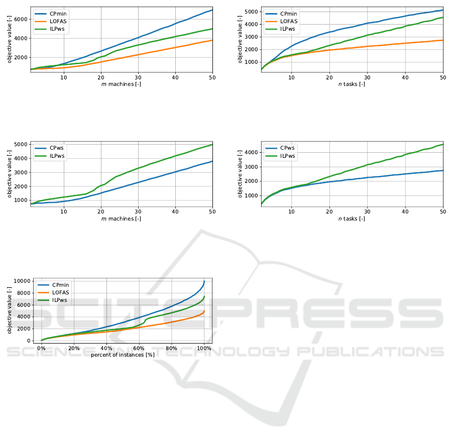
7.2 Results
Figure 5a shows the dependence of the best objective
value found by the exact approaches within the 60s
time limit on the number of machines, averaged over
the various number of tasks. Analogically, Fig. 5b
ICORES 2019 - 8th International Conference on Operations Research and Enterprise Systems
98

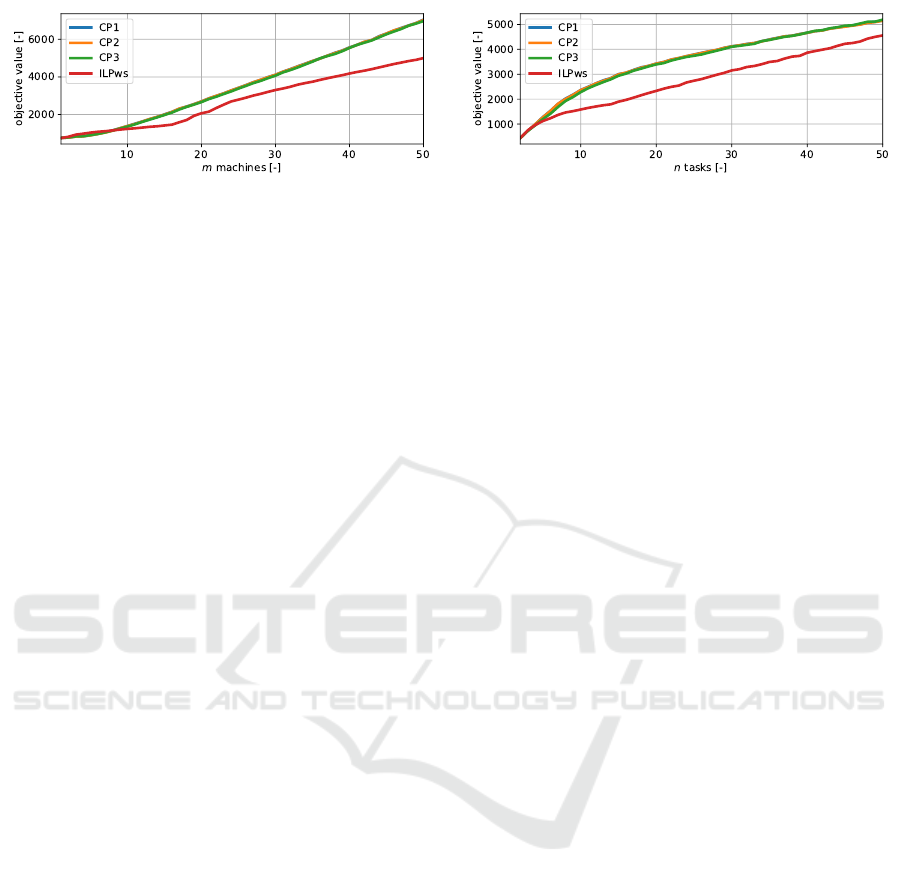
(a) Mean objective value for different number of machines m. (b) Mean objective value for different number of tasks n.
Figure 5: Comparison of exact models.
shows the dependence of the best objective value on
the number of tasks, averaged over the varying num-
ber of machines.
The results show that the performances of CP
models are almost equal (the graphs almost amalga-
mate). We note that CP3 is the best but the advantage
is negligible. Hence, we will not further distinguish
between them and we will use the minimum of all
three CP models that will be referred to as CPmin.
On the other hand, the inclusion of the ILP ap-
proach with the warm starts (henceforth referred to as
ILPws) in this comparison is inappropriate in that the
CP models do not get any warm start. When the ILP
approach model did not get the initial solution as a
warm start, it was not able to find any solution even
for very small instances (i.e., 2 machines and 8 tasks).
In fact, the objective value found by the ILPws is of-
ten the objective value of the greedy initial solution
given as the warm start (i.e., Section 4.2).
Further, we compare the best objective value
found by the heuristic algorithm LOFAS from Sec-
tion 6 against CPmin. Figure 6a shows the depen-
dence on the number of machines, while Fig. 6b
shows the dependence on the number of tasks. Note
that we omit the results of CP3ws (CP3 model with
warm starts) in Fig. 6 as the results were almost the
same as those of LOFAS and the curves amalgamated.
To further compare LOFAS to CP3ws, we gener-
ated instances of size up to 120 tasks on each ma-
chine (119 × 50 = 5950 instances in total). The op-
timality of a solution was proved by CP3ws in to-
tal for 75 instances, and out of these 75 instances,
LOFAS rendered worse solution only for 6 instances,
thus giving an optimal solution in 92 % of instances.
The smallest instance for which CP3ws did not find
any solution consisted of 50 machines and 72 tasks
on each machine, whereas the smallest instance for
which LOFAS did not find any solution contained 117
tasks on each machine. Out of these 5950 instances,
CP3ws did not find any solution for 1018 instances,
while LOFAS did not find any solution only for 53
instances. From instances that were solved by both
algorithms, CP3ws yielded a better solution than LO-
FAS only for 641 instances, whereas LOFAS gave a
better solution than CP3ws for 2329 instances. Fi-
nally, the biggest difference in the objective values
found was 3.74 % in favor of LOFAS, but only 2.45 %
in favor of CP3ws.
The reason why LOFAS did not find any solution
to the biggest instances was that the time limit was ex-
ceeded during the decomposition phase, i.e., during
seeking an optimal sequence for a machine. Hence,
the performance of LOFAS can be significantly im-
proved if a better TSP solver, e.g., Concorde (Apple-
gate et al., 2011), would be used instead of the model
from Section 4.1. This is not the case for CP3ws,
which did not manage to combine the solutions to the
subproblems together already for smaller instances.
Note that the comparison of CP3ws to ILPws,
which is shown in Fig. 7, is legit, as they both get
a warm start in a certain sense, and confirms lower
performance of the ILP approach.
To obtain better insight into the performance of
the proposed methods, we compared the resulting dis-
tributions of achieved objectives from each method.
For each method, we took results for all instances and
ordered them in a non-decreasing way with respect to
achieved objective value and plotted them. The re-
sults are displayed in Fig. 8. It can be seen that the
proposed heuristic is able to find the same or better
solutions in nearly all cases. Moreover, one can no-
tice a spike at around 65 % of instances for ILPws.
This is caused by the fact that for some instances,
the ILP solver was not able to improve upon the ini-
tial warm start solution in the given time limit and
these instances thus contribute to the distribution with
higher objective values.
7.3 Discussion
We have seen that performances of CP models are al-
most equal with CP3 being the best but its advantage
is negligible. Further, the experiments have shown
that ILP without a warm start cannot find a feasi-
Makespan Minimization with Sequence-dependent Non-overlapping Setups
99

(a) Mean objective value for different number of machines m. (b) Mean objective value for different number of tasks n.
Figure 6: Comparison of exact models and the heuristic algorithm.
(a) Mean objective value for different number of machines m. (b) Mean objective value for different number of tasks n.
Figure 7: Comparison of exact models with warm starts.
Figure 8: Objective distributions of different methods.
ble solution for instances with n ≥ 8 tasks reliably,
whereas with warm starts it was significantly better
than the best CP model without a warm start. The
quality of the solutions from CP with warm starts
is much better than ILP with warm starts, as can be
seen in Fig. 7. As expected, the heuristic algorithm
LOFAS produced the best solutions among all com-
pared methods, although only slightly better than CP3
model with warm starts. From smaller instances it can
be seen that LOFAS achieves objective values quite
close to optimal ones.
8 CONCLUSIONS
In this paper, we tackled the problem of schedul-
ing on dedicated machines with sequence-dependent
non-overlapping setups. We suggested an ILP model,
three variants of a CP model and a heuristic algo-
rithm. The extensive experimental evaluation showed
that all exact models themselves are yielding solu-
tions far from optima within the given time limit of 60
seconds, which proved them inappropriate mainly for
larger instances. However, the proposed heuristic al-
gorithm that combines ILP and CP yields high-quality
solutions in very short computation time. The gist is
that we leveraged the strength of ILP in the shortest
Hamiltonian path problem and the efficiency of CP at
sequencing problems with makespan minimization.
For future work, a more complex problem will be
considered. The main limitation of the model pro-
posed in this paper is that tasks are assumed to be al-
ready assigned to machines. In practice, it may hap-
pen that each task can be processed on some subset
of machines. Also, instead of non-overlapping se-
tups for one machine setter, there may be more ma-
chine setters that must be then treated as a resource
with limited capacity. In addition, this capacity may
vary in time (e.g., to avoid night shifts). Another key
feature of many real-life production problems is the
presence of release times and deadlines or precedence
constraints. For such a problem, finding an initial fea-
sible schedule will be already a non-trivial problem
and the solution approach from Section 4.1 for the
case of a single machine does not work anymore.
Next, before a machine setter can perform a setup,
it may require moving to another machine and prepar-
ing some tools, which may lead to a concept of se-
tups over setups. It would require a setup times ma-
trix of size O(|T |
4
), which does not seem plausible.
However, if we settle for the setup times over setups
ICORES 2019 - 8th International Conference on Operations Research and Enterprise Systems
100

to be determined by the pair of machines where the
two consecutive setups are performed, which yields a
setup times matrix of size only O(m
2
), it could bring
the problem closer to real-life applications.
ACKNOWLEDGEMENTS
This work was supported by the Technology Agency
of the Czech Republic under the National Compe-
tence Center - Cybernetics and Artificial Intelligence
TN01000024, by the EU and the Ministry of Indus-
try and Trade of the Czech Republic under the Project
OP PIK CZ.01.1.02/0.0/0.0/15 019/0004688, and by
SVV project number 260 453.
REFERENCES
Allahverdi, A., Ng, C., Cheng, T. E., and Kovalyov, M. Y.
(2008). A survey of scheduling problems with setup
times or costs. European journal of operational re-
search, 187(3):985–1032.
Applegate, D. and Cook, W. (1991). A computational study
of the job-shop scheduling problem. ORSA Journal
on computing, 3(2):149–156.
Applegate, D. L., Bixby, R. E., Chv
´
atal, V., and Cook, W. J.
(2011). The Traveling Salesman Problem: A Compu-
tational Study. Princeton University Press.
Balas, E. (1968). Project scheduling with resource con-
straints. Technical report, Carnegie-Mellon Univ
Pittsburgh Pa Management Sciences Research Group.
Chen, D., Luh, P. B., Thakur, L. S., and Moreno Jr, J.
(2003). Optimization-based manufacturing schedul-
ing with multiple resources, setup requirements, and
transfer lots. IIE Transactions, 35(10):973–985.
Gurobi (2018). Constraints. http://www.gurobi.com/docu-
mentation/8.0/refman/constraints.html. Accessed
September 18, 2018.
Hentenryck, P. V. and Michel, L. (2009). Constraint-based
local search. The MIT press.
Laborie, P., Rogerie, J., Shaw, P., and Vil
´
ım, P. (2009). Rea-
soning with conditional time-intervals. part ii: An al-
gebraical model for resources. In FLAIRS conference,
pages 201–206.
Laborie, P., Rogerie, J., Shaw, P., and Vil
´
ım, P. (2018).
IBM ILOG CP optimizer for scheduling. Constraints,
23(2):210–250.
Lasserre, J. B. and Queyranne, M. (1992). Generic schedul-
ing polyhedra and a new mixed-integer formulation
for single-machine scheduling. Proceedings of the
2nd IPCO (Integer Programming and Combinatorial
Optimization) conference, pages 136–149.
Lee, Y. H. and Pinedo, M. (1997). Scheduling jobs
on parallel machines with sequence-dependent setup
times. European Journal of Operational Research,
100(3):464–474.
Pferschy, U. and Stan
ˇ
ek, R. (2017). Generating subtour
elimination constraints for the TSP from pure integer
solutions. Central European Journal of Operations
Research, 25(1):231–260.
Pisinger, D. and Ropke, S. (2010). Large neighborhood
search. In Handbook of metaheuristics, pages 399–
419. Springer.
Ruiz, R. and Andr
´
es-Romano, C. (2011). Scheduling
unrelated parallel machines with resource-assignable
sequence-dependent setup times. The International
Journal of Advanced Manufacturing Technology,
57(5-8):777–794.
Tempelmeier, H. and Buschk
¨
uhl, L. (2008). Dynamic multi-
machine lotsizing and sequencing with simultaneous
scheduling of a common setup resource. International
Journal of Production Economics, 113(1):401–412.
Vallada, E. and Ruiz, R. (2011). A genetic algorithm for the
unrelated parallel machine scheduling problem with
sequence dependent setup times. European Journal of
Operational Research, 211(3):612–622.
Vil
´
ım, P., Bart
´
ak, R., and
ˇ
Cepek, O. (2005). Extension
of O(n log n) filtering algorithms for the unary re-
source constraint to optional activities. Constraints,
10(4):403–425.
Zhao, X., Luh, P. B., and Wang, J. (1999). Surrogate gradi-
ent algorithm for lagrangian relaxation. Journal of op-
timization Theory and Applications, 100(3):699–712.
Makespan Minimization with Sequence-dependent Non-overlapping Setups
101