
Local LUT Upsampling for Acceleration of Edge-preserving Filtering
Hiroshi Tajima, Teppei Tsubokawa, Yoshihiro Maeda and Norishige Fukushima
∗
Nagoya Institute of Technology, Japan
∗
https://fukushima.web.nitech.ac.jp/en/
Keywords:
Edge-preserving Filtering, Local LUT Upsampling, Acceleration, Bilateral Filtering, L
0
Smoothing.
Abstract:
Edge-preserving filters have been used in various applications in image processing. As the number of pixels
of digital cameras has been increasing, the computational cost becomes higher, since the order of the filters
depends on the image size. There are several acceleration approaches for the edge-preserving filtering; howe-
ver, most approaches reduce the dependency of filtering kernel size to the processing time. In this paper, we
propose a method to accelerate the edge-preserving filters for high-resolution images. The method subsam-
ples an input image and then performs the edge-preserving filtering on the subsampled image. Our method
then upsamples the subsampled image with the guidance, which is the high-resolution input images. For this
upsampling, we generate per-pixel LUTs for high-precision upsampling. Experimental results show that the
proposed method has higher performance than the conventional approaches.
1 INTRODUCTION
Edge-preserving filtering smooths images while
maintaining the outline in the images. There are
various edge-preserving filters for various purposes
of image processing, such as bilateral filtering (To-
masi and Manduchi, 1998), non-local means filte-
ring (Buades et al., 2005), DCT filtering (Yu and
Sapiro, 2011), BM3D (Dabov et al., 2007), guided
image filtering (He et al., 2010), domain transform
filtering (Gastal and Oliveira, 2011), adaptive mani-
fold filtering (Gastal and Oliveira, 2012), local Lapla-
cian filtering (Paris et al., 2011), weighted least square
filtering (Levin et al., 2004), and L
0
smoothing (Xu
et al., 2011). The applications of the edge-preserving
filters include noise removal (Buades et al., 2005),
outline emphasis (Bae et al., 2006), high dynamic
range imaging (Durand and Dorsey, 2002), haze re-
moving (He et al., 2009), stereo matching (Hosni
et al., 2013; Matsuo et al., 2015), free viewpoint
imaging (Kodera et al., 2013), depth map enhance-
ment (Matsuo et al., 2013).
The computational cost of edge-preserving filte-
ring is the main issue. There are several accelera-
tion approaches for each filter, such as bilateral fil-
tering (Durand and Dorsey, 2002; Yang et al., 2009;
Adams et al., 2010; Chaudhury et al., 2011; Chaud-
hury, 2011; Chaudhury, 2013; Sugimoto and Kamata,
2015; Sugimoto et al., 2016; Ghosh et al., 2018; Ma-
eda et al., 2018b; Maeda et al., 2018a), non-local me-
Subsampling
Edge-preserving
smoothing filter
Reference
Output
Generating
Local LUT
Low-resolution
Input
Low-resolution
Output
Input Image Output Image
Local LUT
Figure 1: Local LUT upsampling: an input image is do-
wnsampled and then the image is smoothed by arbitrary
edge-preserving filtering. Next, we create per-pixel LUT
by using the correspondence between subsampled input and
output images. Finally, we convert the input image into the
approximated image by the LUT.
ans filtering (Adams et al., 2010; Fukushima et al.,
2015), local Laplacian filtering (Aubry et al., 2014),
DCT filtering (Fujita et al., 2015), guided image filte-
ring (Murooka et al., 2018; Fukushima et al., 2018b)
and weighted least square filtering (Min et al., 2014).
The computational time of each filter, however, de-
pends on image resolution, and it is rapidly incre-
asing, e.g., smartphone’s cameras even have 12M
pixels. For such a high-resolution image, we require
more acceleration techniques.
Processing with subsampling and then upsam-
pling is the most straightforward approach to acce-
lerate image processing. This approach dramatically
reduces processing time; however, the accuracy of the
Tajima, H., Tsubokawa, T., Maeda, Y. and Fukushima, N.
Local LUT Upsampling for Acceleration of Edge-preserving Filtering.
DOI: 10.5220/0007364601310138
In Proceedings of the 14th International Joint Conference on Computer Vision, Imaging and Computer Graphics Theory and Applications (VISIGRAPP 2019), pages 131-138
ISBN: 978-989-758-354-4
Copyright
c
2019 by SCITEPRESS – Science and Technology Publications, Lda. All rights reserved
131

approximation is also significantly decreased. Subs-
ampling loses high-frequency and large edges in ima-
ges; hence, the resulting images also lose the infor-
mation. Different from super-resolution problems,
subsampling/upsampling for acceleration can utilize
a high-resolution input image as a guidance signal.
Joint bilateral upsampling (Kopf et al., 2007) and gui-
ded image upsampling (He and Sun, 2015) utilize the
high-resolution image for high-quality upsampling as
extensions of joint bilateral filtering (Petschnigg et al.,
2004; Eisemann and Durand, 2004). However, both
upsampling are specific for accelerating bilateral filte-
ring and guided image filtering. Note that More spe-
cific upsampling, e.g., depth map upsampling (Fukus-
hima et al., 2016), improve the upsampling quality.
In this paper, we propose a method to accelerate
arbitrary edge-preserving filters by using subsampling
and upsampling with guidance high-resolution ima-
ges. We named the proposed method local LUT ups-
ampling. Figure 1 indicates the overview of the pro-
posed method. In the proposed, edge-preserving filte-
ring, which has the highest cost in the processing, is
performed in the downsampled domain for accelera-
tion. Then our method utilizes high-resolution infor-
mation for accurate upsampling.
2 RELATED WORK
In this section, we review two edge-preserving filters
used in the section of experimental results, i.e., bila-
teral filtering and L
0
smoothing. Also, we introduce
guided image upsampling, which is an acceleration
method for edge-preserving filtering.
2.1 Bilateral Filtering
Bilateral filtering is a standard edge-preserving filte-
ring, and it is one of the finite impulse response (FIR)
filters. The processing of the bilateral filter for an in-
put image I
I
I can be expressed as:
J
J
J
p
p
p
=
∑
q
q
q∈N
p
p
p
f
bf
(p
p
p,q
q
q)I
I
I
q
q
q
∑
q
q
q∈N
p
p
p
f
bf
(p
p
p,q
q
q)
, (1)
where J
J
J is an output image of the bilateral filter, p
p
p and
q
q
q are target and reference pixels, respectively. N
p
p
p
is a
set of the neighboring pixel of the target pixel p
p
p. f
bf
represents a weight function, and it is defined as:
f
bf
(p
p
p,q
q
q)=exp
kp
p
p−q
q
qk
2
2
−2σ
2
s
exp
kI
I
I
p
p
p
−I
I
I
q
q
q
k
2
2
−2σ
2
c
, (2)
where kp
p
p − q
q
qk
2
2
and kI
I
I
p
p
p
− I
I
I
q
q
q
k
2
2
show the difference
of the spatial distance and luminance value between
the target pixel and the reference pixel, respectively.
σ
s
and σ
c
are smoothing parameters for the Gaussian
distributions of the spatial distance and luminance dif-
ference, respectively. The bilateral filter smooths ima-
ges with the range weight in addition to the spatial
weight. As a result, a large weight is given to a refe-
rence pixel whose distance and luminance from target
pixel is close.
2.2 L
0
Smoothing
L
0
smoothing can emphasize rough edges and can re-
duce fine edges. The L
0
smoothing smooths weak
edge-parts in images more strongly than the bilateral
filtering. Therefore, it is useful for extracting edges
and generating non-photorealistic effects. An output
is obtained by solving the following equation:
min
J,h,v
(
∑
p
p
p
(J
J
J
p
p
p
−I
I
I
p
p
p
)
2
+λC(h,v)
+β((∂
x
J
J
J
p
p
p
−h
p
)
2
+(∂
y
J
J
J
p
p
p
−v
p
)
2
)
, (3)
where I
I
I and J
J
J are input and output images, respecti-
vely. h
p
, v
p
are auxiliary variables corresponding
to ∂
x
J
J
J
p
p
p
and ∂
y
J
J
J
p
p
p
, where p
p
p is a target pixel coordi-
nate, respectively. C(h, v) is the number of p
p
p that
|h
p
| + |v
p
| 6= 0, and β is determined from the gradient
of (h,v). In order to solve Eq. (3), it is divided into
two sub-problems. The first is computing J
J
J. Exclu-
ding the term not including J
J
J from Eq. (3), the follo-
wing equation is obtained:
E =
∑
p
J
J
J
p
−I
I
I
p
)
2
+β((∂
x
J
J
J
p
−h
p
)
2
+(∂
y
J
J
J
p
−v
p
)
2
. (4)
J
J
J is obtained by minimizing equation (4). In this met-
hod, derivative operators are diagonalized after the
fast Fourier transform (FFT) for speedup:
J
J
J =F
−1
F (I
I
I)+β(F (∂
x
)
∗
F (h) + F (∂
y
)
∗
F (v))
F (I
I
I)+β(F (∂
x
)
∗
F (∂
x
)+F (∂
y
)
∗
F (∂
y
))
, (5)
where F is the FFT operator and
∗
denotes the com-
plex conjugate. The second is computing (h,v). The
objective function for (h,v) is defined as follows:
E
0
=
∑
p
min
h
p
,v
p
{(h
p
−∂
x
J
J
J
p
p
p
)
2
+(v
p
−∂
y
J
J
J
p
p
p
)
2
+
λ
β
H(|h
p
|+|v
p
|)}, (6)
where H
H
H(|h
p
| + |v
p
|) is a binary function returning 1,
if |h
p
| + |v
p
| 6= 0 and 0 otherwise. When Eq. (6) is
rewritten to the function E
p
of each pixel p
p
p, the follo-
wing expression is obtained.
E
p
= (h
p
−∂
x
J
J
J
p
p
p
)
2
+(v
p
−∂
y
J
J
J
p
p
p
)
2
+
λ
β
H(|h
p
|+|v
p
|), (7)
VISAPP 2019 - 14th International Conference on Computer Vision Theory and Applications
132

Algorithm 1: L
0
Gradient Minimization.
Input: image I, smoothing weight λ, parameters β
0
,
β
max
, and rate κ
Initialization: J ← I,β ← β
0
,i ← 0
repeat
With J
(i)
, solve for h
(i)
p
and v
(i)
p
in Eq. (8)
With h
(i)
and v
(i)
, solver for J
(i+1)
with Eq. (5)
β ← κβ,i + +
until β ≥ β
max
Output: result image J
which reaches its minimum E
∗
p
under the condition:
(h
p
,v
p
)=
(
(0,0) ((∂
x
J
J
J
p
p
p
)
2
+(∂
y
J
J
J
p
p
p
)
2
≤λ/β)
(∂
x
J
J
J
p
p
p
,∂
y
J
J
J
p
p
p
) (otherwise.)
(8)
After computing the minimum energy E
∗
p
for each
pixel p
p
p, calculating
∑
p
E
∗
p
becomes the global opti-
mum for Eq. (6). The alternating minimization al-
gorithm is sketched in Algorithm 1. Parameter β is
automatically adapted for each iteration. β is starting
from a small value β
0
, and then it is multiplied by κ
each time.
2.3 Guided Image Upsampling
We now summarize guided image upsampling. The
upsampling is an extension of the guided image fil-
tering. The filtering converts local patches in an in-
put image by a linear transformation of a guidance
image. Let the guide signal be G, and it is possible to
be G = I, where I is an input image. The output patch
J
p
p
p
should be satisfied for the following relation:
J
p
p
p
= a
k
k
k
G
p
p
p
+ b
k
k
k
,∀p
p
p ∈ ω
k
k
k
, (9)
where k
k
k indicates a center position of a rectangular
patch ω
k
k
k
, and p
p
p indicates a position of a pixel in the
patch. a
k
k
k
and b
k
k
k
are coefficients for the linear trans-
formation. The equation represents the coefficients
linearly convert the guide signals in a patch.
The coefficients are calculated by a linear regres-
sion of the input signal I and Eq. (9),
arg min
a
k
k
k
,b
k
k
k
=
∑
p
p
p∈ω
k
k
k
((a
k
k
k
J
p
p
p
+ b
k
k
k
− I
p
p
p
)
2
+ εa
2
k
k
k
). (10)
The coefficients are estimated as follows:
a
k
k
k
=
cov
k
k
k
(G,I)
var
k
k
k
(G) + ε
, b
k
k
k
=
¯
I
k
k
k
− a
k
k
k
¯
G
k
k
k
, (11)
where ε indicates a parameter of smoothing degree.
¯·
k
k
k
, cov
k
k
k
and var
k
k
k
indicate the mean, variance, and co-
variance values of the patch k
k
k. The coefficients are
overlapping in the output signals; thus, these coeffi-
cients are averaged;
¯a
i
i
i
=
1
|ω|
∑
k
k
k∈ω
p
p
p
a
k
k
k
,
¯
b
i
i
i
=
1
|ω|
∑
k
k
k∈ω
p
p
p
b
k
k
k
, (12)
where | · | indicates the number of elements in the set.
Finally, the output is calculated as follows:
J
i
i
i
= ¯a
i
i
i
G
i
i
i
+
¯
b
i
i
i
. (13)
For color filtering, let input, output and guidance
signals be I
I
I = {I
1
,I
2
,I
3
}, J
n
(n = 1, 2, 3), and G
G
G, re-
spectively. The per-channel output is defined as:
J
n
p
p
p
=
¯
a
a
a
n
p
p
p
T
G
G
G
p
p
p
+
¯
b
n
p
p
p
, (14)
¯
a
a
a
n
p
p
p
=
1
|ω|
∑
k
k
k∈ω
p
p
p
a
a
a
n
k
k
k
,
¯
b
n
p
p
p
=
1
|ω|
∑
k
k
k∈ω
p
p
p
b
n
k
k
k
. (15)
The coefficients a
a
a
n
k
k
k
, b
n
k
k
k
are obtained as follows:
a
a
a
n
k
k
k
=
cov
k
k
k
(G
G
G,I
n
)
var
k
k
k
(G
G
G) + εE
E
E
, b
n
k
k
k
=
¯
I
n
k
k
k
− a
a
a
n
k
k
k
T
¯
G
G
G
k
k
k
, (16)
where E
E
E is an identity matrix. When the output sig-
nal is a color image, cov
k
k
k
is the covariance matrix of
the patch in I and G
G
G. Also, var
k
k
k
is the variance of
the R, G, and B components, which will be covari-
ance matrix, in the patch of G
G
G. The division of the
matrix is calculated by multiplying the inverse matrix
of the denominator from the left. We use box filte-
ring for the calculation of per pixel mean, variance,
and covariance. The fast implementation of the box
filtering (Fukushima et al., 2018a) accelerates the fil-
tering.
The guided image upsampling is an extension of
guided image filtering and the upsampling is expres-
sed as:
J
n
p
p
p
= S
−1
s
(S
s
(
¯
a
a
a
n
p
p
p
)
T
G
G
G
p
p
p
+ S
−1
s
(S
s
(
¯
b
n
p
p
p
)), (17)
where S(·) and S
−1
(·) indicate subsampling and ups-
ampling operators, respectively. The upsampling
computes coefficients of
¯
a
a
a
p
p
p
and
¯
b
p
p
p
in the subsampled
domain, and then upsamples the coefficients. Notice
that we should keep high-resolution signal of G
G
G.
The coefficients in the downsampled domain is
computed as follows:
¯
a
a
a
0
n
p
p
p
↓
:= S(
¯
a
a
a
n
p
p
p
),
¯
b
0
n
p
p
p
↓
:= S(
¯
b
n
p
p
p
), (18)
¯
a
a
a
0
n
p
p
p
↓
=
1
|ω
0
|
∑
k
k
k
↓
∈ω
0
p
p
p
a
a
a
n
k
k
k
↓
,
¯
b
n
p
p
p
↓
=
1
|ω
0
|
∑
k
k
k
↓
∈ω
0
p
p
p
b
n
k
k
k
↓
, (19)
a
a
a
0
n
k
k
k
↓
=
cov
k
k
k
↓
(G
G
G
0
0
0
,I
0n
)
var
k
k
k
↓
(G
G
G
0
0
0
) + εE
E
E
, b
0
n
k
k
k
↓
=
¯
I
0
n
k
k
k
↓
− a
0
n
k
k
k
↓
T
¯
G
G
G
0
0
0
k
k
k
↓
,
(20)
Local LUT Upsampling for Acceleration of Edge-preserving Filtering
133

where p
p
p
↓
indicates pixel coordinate in the downsam-
pled domain. Also, a
a
a
0
and b
0
are coefficients in the
downsampled domain, respectively G
G
G
0
:= S(G
G
G) and
I
0
:= S(I) represent downsampled input and guidance
images, respectively. The filtering radius is reduced
according to the rate of subsampling; thus, ω
0
indica-
tes a small rectangular patch, which is reshaped to fit
the rate of subsampling.
3 PROPOSED METHOD
We propose an upsampling method guided by a high-
resolution image for various edge-preserving filte-
ring. The proposed method generates a per-pixel
look-up table (LUT), which maps pixel values of the
input image to that of the output image of the edge-
preserving filtering. If we have the result of edge-
preserving filtering, we can easily transform the in-
put image into the edge-preserving result by one-to-
one mapping. We generate the mapping function in
the subsampled image domain for acceleration. The
proposed method generates per-pixel LUTs for the
function from the correspondence between a subsam-
pled input and its filtering result.
Luminance values are highly correlated between
pixels and its neighboring region in the image. Also,
the correlation between the output of edge-preserving
filtering and the input image becomes high. There-
fore, in this method, a LUT for each pixel is created
from a pair of low-resolution input and output ima-
ges. Then, we refer the subsampled LUT to generate
the high-resolution edge-preserving image. Initially,
an input image I
I
I is subsampled to generate a low-
resolution input image I
I
I
↓
:
I
I
I
↓
= S
s
(I
I
I), (21)
where S
s
is a subsampling operator. Then, edge-
preserving filter is applied for I
I
I
↓
and the output J
J
J
↓
is obtained as follows:
J
J
J
↓
= F(I
I
I
↓
), (22)
where F is an operator of arbitrary edge-preserving
filtering. Then, we count frequency of one-to-one
mapping between the images J
J
J
↓
and I
I
I
↓
. Let f
p
p
p
(s,t)
be a frequency map on a pixel p
p
p, where s and t are an
intensity value on image I
I
I
↓
and J
J
J
↓
, respectively. The
frequency is counted by gathering around a pixel. The
map f is defined as follows:
f
p
p
p
(s,t) =
∑
q
q
q∈W
p
p
p
δ(S
c
(I
I
I
q
q
q↓
),s)δ(S
c
(J
J
J
q
q
q↓
),t), (23)
S
c
(x) = bx/lc (24)
0
32
64
96
128
0
32
64
96
128
Output
Input
(a) Frequency map
0
32
64
96
128
0
32
64
96
128
Output
Input
(b) Winner-takes-all
0
32
64
96
128
0
32
64
96
128
Output
Input
(c) Dynamic programming
Figure 2: Frequency map f
p
p
p
(s,t) and its results of winner-
takes-all and dynamic programming approaches for local
LUT on p
p
p. The number of bins is 128, i.e., quantization
level is l = 2. The radius is r = 20 for visibility of this
figure. In the experiment, small radius setting, e.g., r = 2, 3
have better performance.
where δ(a,b) indicates the Kronecker delta function.
p
p
p = (x,y) indicates a pixel position in the images of
I
I
I
↓
and J
J
J
↓
. q
q
q is a neighboring pixel around p
p
p. W
p
p
p
indicates the set including q
q
q. S
c
(x) is a quantization
function, which is divided by l. The output values
have 256/l candidates. The redaction also accelera-
tes the processing. We call the number of intensity
candidates as the number of bins.
Next, we determine a local LUT on a pixel p
p
p.
With the simplest solution, we select the maximum
frequency argument from the f by the winner-takes-
all approach (WTA). The LUT under the downsam-
pled domain is defined as follows:
T
p
p
p↓
[s] = arg max
t
f (s,t) (25)
The operator [·] is an array operator in programming
languages, such as C programming language. We
cannot determine the value where f (s,t) = 0|
∀t
. In
this case, we linearly interpolate the values by the ne-
arest non-zero values around s. For boundary con-
dition, we set T
p
p
p↓
[0] = 0 and T
p
p
p↓
[255] = 255, when
f (s,t) = 0|
∀t
. The solution cannot keep monotonicity
for the LUT. The fact sometimes generates negative
edges.
To keep the monotonicity, we can solve the pro-
blem by using dynamic programming (DP). We as-
sume that T
p
p
p
[0] = 0 and T
p
p
p
[n] >= T
p
p
p
[n]. We define a
cost function C(s,t) for the DP under this condition:
VISAPP 2019 - 14th International Conference on Computer Vision Theory and Applications
134

(a) artificial (3072 × 2048) (b) tree (6088 × 4550) (c) bridge (2749× 4049)
(d) cathedral (2000 × 3008) (e) fireworks (3136 × 2352)
Figure 3: High-resolution test images.
C(s,t)= max
C(s−1,t−1) + O,C(s−1,t)),C(s,t−1)
+ f (s,t)
(26)
where C(0, 0) = f (0,0), C(s,t) = 0 (s < 0 ∨ t < 0).
The parameter O represent an offset value to enforce
diagonal matching. The cost function can be recursi-
vely updated. After filling the cost function, then we
trace back the function to determine a solid pass.
T
p
p
p↓
= arg DP
p
p
pa
a
as
s
ss
s
s
C(s,t), (27)
where p
p
pa
a
as
s
ss
s
s shows the tracing back pass of the cost
matrix C by using DP. Figure 2 shows the frequency
map and the resulting LUTs obtained by WTA and
DP. After WTA and DP, the matrix indicates one-to-
one mapping. We call this per-pixel LUT T
p
p
p
as local
LUT.
The LUT has three-dimensional information, such
as n, p
p
p = (x, y); however, all elements are subsampled.
It has not enough to map an input image into a high-
resolution image. Therefore, we upsample the LUT
by using tri-linear upsampling. The upsampling is de-
fined as follows:
T
p
p
p
= S
−1
c
(S
−1
s
(T
p
p
p↓
)), (28)
where S
−1
c
and S
−1
s
is upsampling operator for the in-
tensity and spatial domain, respectively. p
p
p indicates
the image coordinate of pixel in the upsampled dom-
ain.
Finally, the output image is referred from the local
LUT and input intensity I
I
I
p
p
p
. The output is defined by:
J
J
J
p
p
p
= T
p
p
p
[I
I
I
p
p
p
]. (29)
4 EXPERIMENTAL RESULTS
We approximated two edge-preserving filters, such as
iterative bilateral filtering and L
0
smoothing by subs-
ampling based acceleration methods. These filters can
mostly smooth images; however, the computational
cost is high. We compared the proposed method of
the local LUT upsampling with the conventional met-
hod of the cubic upsampling and guided image ups-
ampling by approximation accuracy and computatio-
nal time. Also, we compared the proposed method
with na
¨
ıve implementation, which does not subsam-
ple images, in computational time. We utilized high-
resolution test images, which are shown in Fig. 3
1
.
We used two metrics of PSNR and SSIM (Wang
et al., 2004) for accuracy evaluation, and we regar-
ded the results of the na
¨
ıve filtering as ground truth
1
http://imagecompression.info
Local LUT Upsampling for Acceleration of Edge-preserving Filtering
135
results. We implemented the proposed method by
C++ with OpenMP parallelization. We also used In-
tel IPP for the cubic upsampling, which is optimized
by AVX/AVX2. For guided image upsampling, we
also optimized by AVX/AVX2 with OpenCV functi-
ons. For downsampling in the proposed method, we
use the nearest neighbor downsampling. This downs-
ampling has better performance than the cubic inter-
polation for our method. We used OpenCV and In-
tel IPP for the operation with cv::INTER NN option.
The used computer was Intel Core i7 6700 (3.40 GHz)
and compiled by Visual Studio 2017. We used r = 3
for local LUT upsampling, r = 10, iteration = 10,
σ
s
= 10,σ
c
= 20 for iterative bilateral filtering, and
λ = 0.01 and κ = 1.5 for L
0
smoothing.
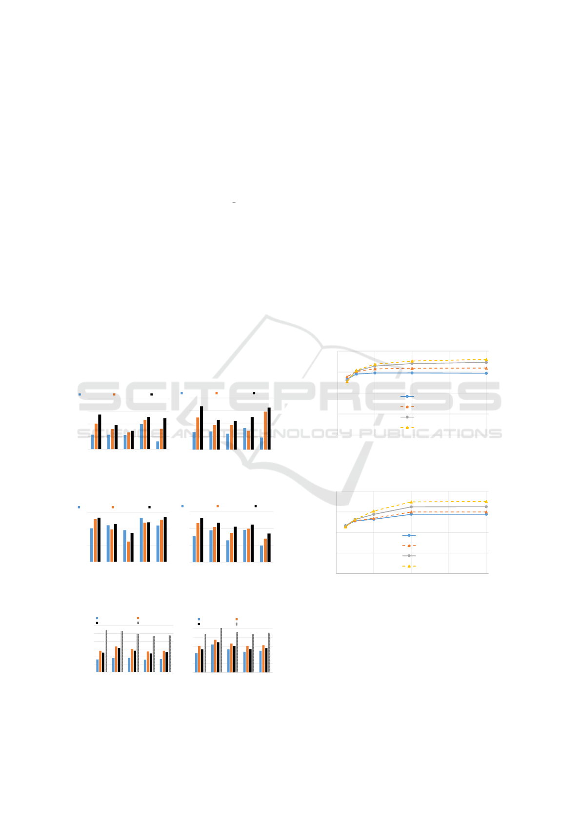
Figures 4, 5, and 6 show the PSNR/SSIM accu-
racy and computational time of iterative bilateral fil-
tering and L
0
smoothing for large images. The para-
meters of the proposed method are l = 2 and downs-
ampling ratio is 8 × 8. The computational time is an
average of 10 trails. The local LUT upsampling has
drastically higher PSNR than the cubic interpolation
for each image. Guided image upsampling is slower
and lower PSNR than the proposed method. The com-
putation time of the local LUT is ×100 faster than the
na
¨
ıve implementation; however, the cubic upsampling
20
25
30
35
40
artificial
tree
bridge
cathedral
fireworks
PSNR [dB]
cubic upsampling
guided upsampling
local LUT
(a) Bilateral filtering
20
25
30
35
40
artificial
tree
bridge
cathedral
fireworks
PSNR [dB]
cubic upsampling
guided upsampling
local LUT
(b) L
0
smoothing
Figure 4: Approximation accuracy of PSNR for each image
and method.
0.7
0.8
0.9
1.0
artificial
tree
bridge
cathedral
fireworks
SSIM
cubic upsampling
guided upsampling
local LUT
(a) Bilateral filtering
0.7
0.8
0.9
1.0
artificial
tree
bridge
cathedral
fireworks
SSIM
cubic upsampling
guided upsampling
local LUT
(b) L
0
smoothing
Figure 5: Approximation accuracy of SSIM for each image
and method.
1
10
100
1000
10000
100000
1000000
artificial
tree
bridge
cathedral
fireworks
Time [ms]
cubic upsampling
guided upsampling
local LUT
naive
(a) Bilateral filtering
1
10
100
1000
10000
100000
artificial
tree
bridge
cathedral
fireworks
Time [ms]
cubic upsampling
guided upsampling
local LUT
naive
(b) L
0
smoothing
Figure 6: Computational time for each image and method.
is ×10000 faster. Notice that the code of the proposed
method is not vectorized, such as AVX/AVX2; thus,
the proposed can speed up by programming, while In-
tel’s code fully optimizes the cubic upsampling. We
now optimize the code for the proposed method while
reviewing period.
Figures 7 and 8 show the relationship between
spatial/range subsampling ratio and PSNR for itera-
tive bilateral filtering and L
0
smoothing. The result
shows that 1/4 range downsampling (64 bin) and
8 × 8 spatial downsampling do not notable decrease
the PSNR quality.
Figures 9 and 10 show the trade-off between the
PSNR accuracy and computational time by changing
the resizing ratio from 1/16 to 1/1024. We also
change the number of bins for local LUT upsampling.
These results show that the proposed method has the
best trade-off than the cubic interpolation and guided
image upsampling.
Figures 11 and 12 depict input image and results
of each upsampling method for iterative bilateral fil-
tering and L
0
smoothing, respectively.
15
20
25
30
35
0
32
64
96
128
PSNR [dB]
number of bins
subsampling rate : 1024
subsampling rate : 256
subsampling rate : 64
subsampling rate : 16
Figure 7: Bilateral filtering result: PSNR w.r.t. the number
of bins with changing resizing ratio.
20
25
30
35
40
0
32
64
96
128
PSNR [dB]
number of bins
subsampling rate : 1024
subsampling rate : 256
subsampling rate : 64
subsampling rate : 16
Figure 8: L
0
smoothing result: PSNR w.r.t. the number of
bins with changing resizing ratio.
5 CONCLUSIONS
In this paper, we proposed an acceleration method for
edge-preserving filtering with image upsampling. We
call the upsampling as local LUT upsampling. The lo-
VISAPP 2019 - 14th International Conference on Computer Vision Theory and Applications
136
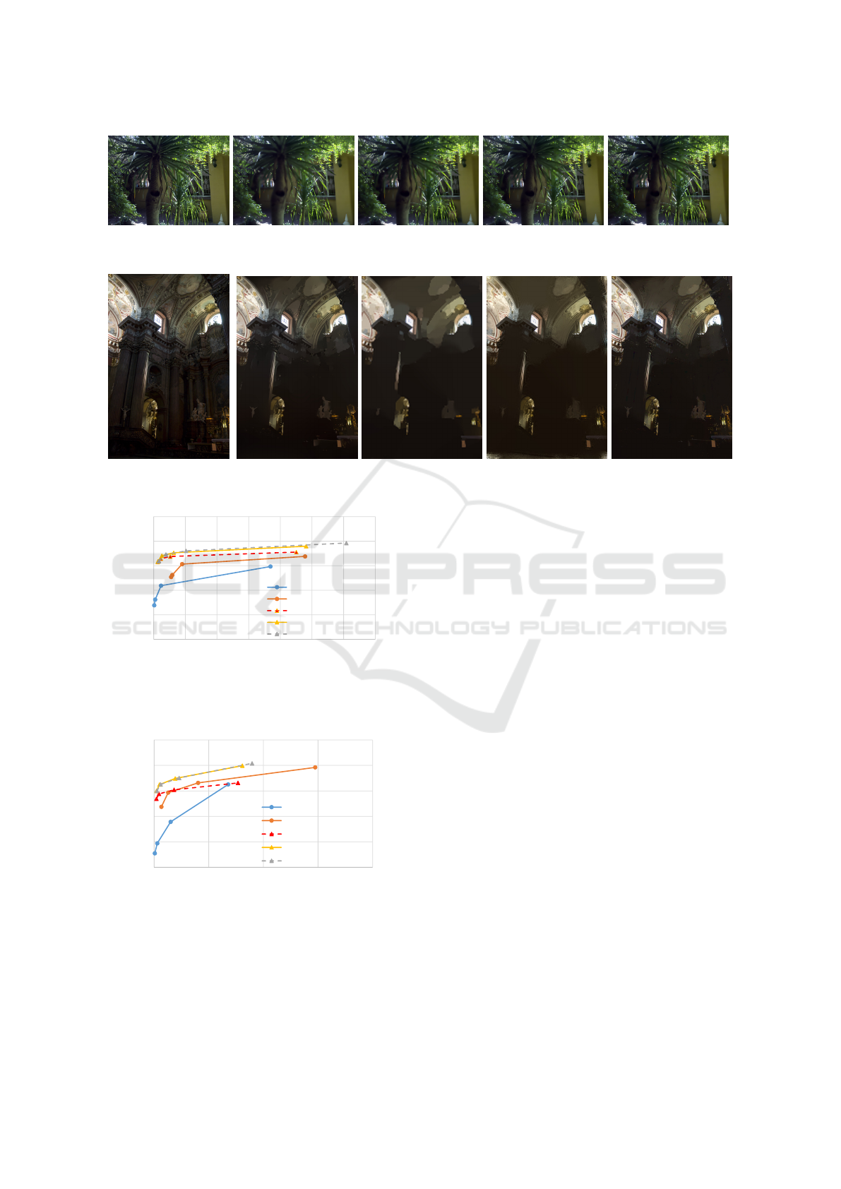
(a) Input (b) Na
¨
ıve (c) Cubic (d) Guided Upsampling (e) Local LUT
Figure 11: Results of iterative bilateral filtering.
(a) Input (b) Na
¨
ıve (c) Cubic (d) Guided Upsampling (e) Local LUT
Figure 12: Results of L
0
smoothing.
15
20
25
30
35
40
0
1000
2000
3000
4000
5000
6000
7000
PSNR [dB]
Time [ms]
cubic upsampling
guided upsampling
number of bins : 32
number of bins : 64
number of bins : 128
Figure 9: Resizing and changing the number of bins perfor-
mance in PSNR w.r.t. computational time (bilateral filter).
Local LUT samples 32, 64, and 128 bins, respectively.
20
25
30
35
40
45
0
5000
10000
15000
20000
PSNR [dB]
Time [ms]
cubic upsampling
guided upsampling
number of bins : 32
number of bins : 64
number of bins : 128
Figure 10: Resizing and changing the number of bins per-
formance in PSNR w.r.t. computational time (L
0
smoo-
thing). Local LUT samples 32, 64, and 128 bins, respecti-
vely.
cal LUT upsampling has higher approximation accu-
racy than the conventional approaches of cubic and
guided image upsampling. Also, the local LUT ups-
ampling accelerates ×100 faster than the na
¨
ıve imple-
mentation.
ACKNOWLEDGEMENTS
This work was supported by JSPS KAKENHI
(JP17H01764, 18K18076).
REFERENCES
Adams, A., Baek, J., and Davis, M. A. (2010). Fast high-
dimensional filtering using the permutohedral lattice.
Computer Graphics Forum, 29(2):753–762.
Aubry, M., Paris, S., Hasinoff, S. W., Kautz, J., and Durand,
F. (2014). Fast local laplacian filters: Theory and ap-
plications. ACM Transactions on Graphics, 33(5).
Bae, S., Paris, S., and Durand, F. (2006). Two-scale tone
management for photographic look. ACM Transacti-
ons on Graphics, pages 637–645.
Buades, A., Coll, B., and Morel, J. M. (2005). A non-local
algorithm for image denoising. In Proc. Computer Vi-
sion and Pattern Recognition (CVPR).
Chaudhury, K. N. (2011). Constant-time filtering using
shiftable kernels. IEEE Signal Processing Letters,
18(11):651–654.
Chaudhury, K. N. (2013). Acceleration of the shiftable o(1)
algorithm for bilateral filtering and nonlocal means.
IEEE Transactions on Image Processing, 22(4):1291–
1300.
Chaudhury, K. N., Sage, D., and Unser, M. (2011).
Fast o(1) bilateral filtering using trigonometric range
Local LUT Upsampling for Acceleration of Edge-preserving Filtering
137

kernels. IEEE Transactions on Image Processing,
20(12):3376–3382.
Dabov, K., Foi, A., Katkovnik, V., and Egiazarian, K.
(2007). Image denoising by sparse 3-d transform-
domain collaborative filtering. IEEE Transactions on
image processing, 16(8):2080–2095.
Durand, F. and Dorsey, J. (2002). Fast bilateral filtering
for the display of high-dynamic-range images. ACM
Transactions on Graphics, 21(3):257–266.
Eisemann, E. and Durand, F. (2004). Flash photography en-
hancement via intrinsic relighting. ACM Transactions
on Graphics, 23(3):673–678.
Fujita, S., Fukushima, N., Kimura, M., and Ishibashi, Y.
(2015). Randomized redundant dct: Efficient denoi-
sing by using random subsampling of dct patches. In
Proc. ACM SIGGRAPH Asia 2015 Technical Briefs.
Fukushima, N., Fujita, S., and Ishibashi, Y. (2015). Swit-
ching dual kernels for separable edge-preserving fil-
tering. In Proc. IEEE International Conference on
Acoustics, Speech and Signal Processing (ICASSP).
Fukushima, N., Maeda, Y., Kawasaki, Y., Nakamura, M.,
Tsumura, T., Sugimoto, K., and Kamata, S. (2018a).
Efficient computational scheduling of box and gaus-
sian fir filtering for cpu microarchitecture. In Proc.
Asia-Pacific Signal and Information Processing As-
sociation Annual Summit and Conference (APSIPA),
2018.
Fukushima, N., Sugimoto, K., and Kamata, S. (2018b).
Guided image filtering with arbitrary window
function. In Proc. IEEE International Conference on
Acoustics, Speech and Signal Processing (ICASSP).
Fukushima, N., Takeuchi, K., and Kojima, A. (2016). Self-
similarity matching with predictive linear upsampling
for depth map. In Proc. 3DTV-Conference.
Gastal, E. S. L. and Oliveira, M. M. (2011). Domain
transform for edge-aware image and video processing.
ACM Transactions on Graphics, 30(4).
Gastal, E. S. L. and Oliveira, M. M. (2012). Adaptive ma-
nifolds for real-time high-dimensional filtering. ACM
Transactions on Graphics, 31(4).
Ghosh, S., Nair, P., and Chaudhury, K. N. (2018). Optimi-
zed fourier bilateral filtering. IEEE Signal Processing
Letters, 25(10):1555–1559.
He, K. and Sun, J. (2015). Fast guided filter. CoRR,
abs/1505.00996.
He, K., Sun, J., and Tang, X. (2009). Single image haze
removal using dark channel prior. In Proc. Computer
Vision and Pattern Recognition (CVPR).
He, K., Sun, J., and Tang, X. (2010). Guided image fil-
tering. In Proc. European Conference on Computer
Vision (ECCV).
Hosni, A., Rhemann, C., Bleyer, M., Rother, C., and Ge-
lautz, M. (2013). Fast cost-volume filtering for vi-
sual correspondence and beyond. IEEE Transacti-
ons on Pattern Analysis and Machine Intelligence,
35(2):504–511.
Kodera, N., Fukushima, N., and Ishibashi, Y. (2013). Fil-
ter based alpha matting for depth image based ren-
dering. In Proc. IEEE Visual Communications and
Image Processing (VCIP).
Kopf, J., Cohen, M. F., Lischinski, D., and Uyttendaele, M.
(2007). Joint bilateral upsampling. ACM Transactions
on Graphics, 26(3).
Levin, A., Lischinski, D., and Weiss, Y. (2004). Colo-
rization using optimization. ACM Transactions on
Graphics, 23(3):689–694.
Maeda, Y., Fukushima, N., and Matsuo, H. (2018a). Ef-
fective implementation of edge-preserving filtering on
cpu microarchitectures. Applied Sciences, 8(10).
Maeda, Y., Fukushima, N., and Matsuo, H. (2018b). Taxo-
nomy of vectorization patterns of programming for fir
image filters using kernel subsampling and new one.
Applied Sciences, 8(8).
Matsuo, T., Fujita, S., Fukushima, N., and Ishibashi, Y.
(2015). Efficient edge-awareness propagation via
single-map filtering for edge-preserving stereo mat-
ching. In Proc. SPIE, volume 9393.
Matsuo, T., Fukushima, N., and Ishibashi, Y. (2013). Weig-
hted joint bilateral filter with slope depth compensa-
tion filter for depth map refinement. In Proc. Inter-
national Conference on Computer Vision Theory and
Applications (VISAPP).
Min, D., Choi, S., Lu, J., Ham, B., Sohn, K., and Do, M. N.
(2014). Fast global image smoothing based on weig-
hted least squares. IEEE Transactions on Image Pro-
cessing, 23(12):5638–5653.
Murooka, Y., Maeda, Y., Nakamura, M., Sasaki, T., and Fu-
kushima, N. (2018). Principal component analysis for
acceleration of color guided image filtering. In Proc.
International Workshop on Frontiers of Computer Vi-
sion (IW-FCV).
Paris, S., Hasinoff, S. W., and Kautz, J. (2011). Local lapla-
cian filters: Edge-aware image processing with a lap-
lacian pyramid. pages 68:1–68:12.
Petschnigg, G., Agrawala, M., Hoppe, H., Szeliski, R., Co-
hen, M., and Toyama, K. (2004). Digital photography
with flash and no-flash image pairs. ACM Transacti-
ons on Graphics, 23(3):664–672.
Sugimoto, K., Fukushima, N., and Kamata, S. (2016).
Fast bilateral filter for multichannel images via soft-
assignment coding. In Proc. Asia-Pacific Signal and
Information Processing Association Annual Summit
and Conference (APSIPA).
Sugimoto, K. and Kamata, S. (2015). Compressive bilate-
ral filtering. IEEE Transactions on Image Processing,
24(11):3357–3369.
Tomasi, C. and Manduchi, R. (1998). Bilateral filtering for
gray and color images. In Proc. International Confe-
rence on Computer Vision (ICCV), pages 839–846.
Wang, Z., Bovik, A. C., Sheikh, H. R., and Simoncelli, E. P.
(2004). Image quality assessment: from error visi-
bility to structural similarity. IEEE Transactions on
Image Processing, 13(4):600–612.
Xu, L., Lu, C., Xu, Y., and Jia, J. (2011). Image smoothing
via l0 gradient minimization. ACM Transactions on
Graphics.
Yang, Q., Tan, K. H., and Ahuja, N. (2009). Real-time o
(1) bilateral filtering. In Proc. Computer Vision and
Pattern Recognition (CVPR), pages 557–564.
Yu, G. and Sapiro, G. (2011). Dct image denoising: A sim-
ple and effective image denoising algorithm. Image
Processing On Line, 1:1.
VISAPP 2019 - 14th International Conference on Computer Vision Theory and Applications
138
