Hyperparameter Optimization for Deep Reinforcement Learning in

Vehicle Energy Management

Roman Liessner, Jakob Schmitt, Ansgar Dietermann and Bernard B

aker

Dresden Institute of Automobile Engineering, TU Dresden, George-B

ahr-Straße 1c, 01069 Dresden, Germany

Keywords:

Deep Reinforcement Learning, Hyperparameter Optimization, Random Forest, Energy Management, Hybrid

Electric Vehicle.

Abstract:

Reinforcement Learning is a framework for algorithms that learn by interacting with an unknown environ-

ment. In recent years, combining this approach with deep learning has led to major advances in various ﬁelds.

Numerous hyperparameters – e.g. the learning rate – inﬂuence the learning process and are usually determined

by testing some variations. This selection strongly inﬂuences the learning result and requires a lot of time and

experience. The automation of this process has the potential to make Deep Reinforcement Learning available

to a wider audience and to achieve superior results. This paper presents a model-based hyperparameter op-

timization of the Deep Deterministic Policy Gradients (DDPG) algorithm and demonstrates it with a hybrid

vehicle energy management environment. In the given case, the hyperparameter optimization is able to double

the gained reward value of the DDPG agent.

1 INTRODUCTION

1.1 Motivation and Relevance

In recent years, machine learning has made great

progress in various domains. Particularly in the area

of supervised learning, numerous successes have

been recorded, including the image classiﬁcation

(Krizhevsky et al., 2012), speech recognition (Graves

et al., 2013) and machine translation (Sutskever et al.,

2014). Deep Reinforcement Learning (DRL) gained

media attention by defeating the Go World Champion

(Silver et al., 2017) and playing ATARI games

on an advanced human level (Mnih et al., 2015).

Compared to supervised learning, reinforcement

learning is currently more the subject of research than

of industrial applications (Mania et al., 2018). The

DRL learning process requires numerous pre-deﬁned

parameters. These ensure that the DRL algorithm can

learn on its own during the learning process through

interaction with an environment. These parameters

known as hyperparameters are for example learning

rates, neural network size, exploration and others.

They are not automatically tuned during training.

The user has to select them according to his experi-

ence. The result of the learning process and thus of

the according environment interaction as well as the

required learning time strongly depend on this choice.

A common method is the manual search for suit-

able parameters. Sufﬁcient expertise and experience

are required to ﬁnd good hyperparameter sets. How-

ever, ﬁnding the optimal hyperparameters is usually

unlikely (Chollet, 2017). The introduction of an auto-

mated hyperparameter search process offers two ma-

jor advances. First, the universal industrial applica-

tion can be advanced, as the user is not reliant on

sophisticated personal experience regarding the tun-

ing of hyperparameters. Second, the optimality-based

problem solving using DRL algorithms can be ad-

vanced into a true optimization, as only the identi-

ﬁcation of the optimal hyperparameters enable the

DRL algorithms to deliver optimal results regarding

the given task.

1.2 Related Work

Grid search is a traditional approach to ﬁnd suitable

hyperparameters. A reasonable subset of values is de-

ﬁned for each hyperparameter. Each value combina-

tion is evaluated against a deﬁned validation problem

and ﬁnally the combination achieving the best results

is used in the actual learning task. This method is

easy to implement and a widely used approach for

the optimization of parameters. Duan et al. optimize

the hyperparameters of different RL algorithms using

134

Liessner, R., Schmitt, J., Dietermann, A. and Bäker, B.

Hyperparameter Optimization for Deep Reinforcement Learning in Vehicle Energy Management.

DOI: 10.5220/0007364701340144

In Proceedings of the 11th International Conference on Agents and Artiﬁcial Intelligence (ICAART 2019), pages 134-144

ISBN: 978-989-758-350-6

conventional grid search (Duan et al., 2016). Mania

et al. apply grid search as well to ﬁne-tune their op-

timization algorithm (Mania et al., 2018). Besides

the random parameters selection, choosing promis-

ing parameter combinations based on Bayesian meth-

ods represents an alternative approach. Barsce et al.

use a Gaussian process as underlying model of their

Bayesian method (Barsce et al., 2018). They opti-

mize the hyperparameters of the SARSA(λ) RL al-

gorithm, applied to a simple example of a blocking

maze (Sutton and Barto, 2012). Falkner et al. make

use of the Tree Parzen Estimator as a basic function

of their Bayesian optimization and combine its effec-

tiveness with the speed of the Bandit Random Search

(Falkner et al., 2018). Springenberg et al. approxi-

mate the Bayesian model with the help of neuronal

nets (Springenberg et al., 2016). Both papers exam-

ine the hyperparameter optimization of RL algorithms

using the Cartpole Swing-Up environment as example

case.

These approaches optimize the hyperparameters

of Reinforcement Learning methods which are used

to control physical systems within research demos.

This paper presents a model-based hyperparameter

optimization which is applied to an industrial real

world example. In contrast to demo problems, the

industrial application demands further requirements

such as a limitation of the time, in which the algorithm

has performed the learning process. In this contri-

bution, the hyperparameter optimization is extended

with a hard requirement on the time available for the

learning process of the DDPG algorithm in its indus-

trial application. It is shown, how well the hyperpa-

rameter optimization tunes the DDPG to achieve re-

sults, which extend the results gained with a hyperpa-

rameter set manually deﬁned by experts, while simul-

taneously complying to the time requirements.

1.3 Structure of this Paper

Chapter two of this paper gives an introduction into

Deep RL algorithms and the hyperparameters which

are included in the optimization process. Chapter

three will provide more information on the previously

described hyperparameter optimization approaches.

Also, three methods are selected for further study in

the context of this paper, with focus on the model-

based approaches. Chapter four describes the envi-

ronment, which the Deep RL agent is interacting with

and which represents the vehicle energy management

problem. Chapter ﬁve analyses the achieved results

with the selected hyperparameter optimization meth-

ods, followed by the conclusion in chapter six.

Figure 1: Agent-Environment-Interaction of Reinforcement

Learning (Sutton and Barto, 1998).

2 BACKGROUND

2.1 Reinforcement Learning

Reinforcement Learning is a direct approach to learn

from interactions with an environment in order to

achieve a deﬁned goal. The basic interaction is shown

in Figure 1. In this context, the learner and decision

maker is referred to as the agent, whereas the part it

is interacting with is called environment. The interac-

tion performs in a continuous form so that the agent

selects actions A

at each time step t, the environment

responds to them and presents new situations (in the

form of a state S

t+1

) to the agent

. Responding to

the agent’s feedback, the environment returns rewards

t+1

in the form of a numerical scalar value. The

agent seeks to maximize rewards over time (Sutton

and Barto, 1998).

Having introduced the idea of the RL, a brief ex-

planation of certain terms follows. For a detailed in-

troduction, please refer to (Sutton and Barto, 1998).

Policy: The policy, is what characterizes the agents

behavior. More formally the policy is a mapping from

states to actions.

π(a|s) = P(A

= a|S

= s) (1)

Goals and Rewards: In reinforcement learning, the

agent’s goal is formalized in the form of a special sig-

nal called a reward, that is transferred from the envi-

ronment to the agent at each time step. Basically, the

target of the agent is to maximize the total amount of

scalar rewards R

∈ R it receives. This means maxi-

mizing not the immediate reward, but the cumulative

reward in the long run, which is also called return.

In engineering applications, the agent is the controller,

the environment is the technical system to be inﬂuenced and

the action is the control signal. Nevertheless, the following

deliberately retains the established terms for reinforcement

learning in order to prevent misunderstandings and to pro-

vide the topic to a broader audience in the usual form.

Hyperparameter Optimization for Deep Reinforcement Learning in Vehicle Energy Management

135

Exploration vs. Exploitation: A major challenge

in reinforcement learning is the balance of exploration

and exploitation. In order to receive high rewards, the

agent has to choose actions that have proven to be par-

ticularly rewarding in the past. In order to discover

such actions in the ﬁrst place, new actions have to be

tested. This means the agent has to exploit knowl-

edge already learned to get a reward, and at the same

time explore other actions to have a better strategy

in the future (Sutton and Barto, 1998). Various ex-

ploration strategies are available for this purpose. In

(Plappert et al., 2017), M. Plappert compares several

exploration strategies for continuous action spaces.

In numerous articles (Lillicrap et al., 2015) (Plap-

pert et al., 2017) a correlated additive Gaussian ac-

tion noise based on the Ornstein-Uhlenbeck process

(OUP) (Uhlenbeck and Ornstein, 1930) is applied.

The stochastic process models the velocity of a Brow-

nian particle with friction, resulting in temporally cor-

related values around zero. Compared to the uncorre-

lated additive Gaussian action noise, the action noise

changes less abruptly from one timestep to the next

(Lillicrap et al., 2015). This characteristic can be ben-

eﬁcial for the control of physical actuators. M. Plap-

pert points out in (Plappert et al., 2017), that an addi-

tional action noise is not (always) mandatory in con-

tinuous action spaces. This fact will be discussed in

more detail in the following.

2.2 Deep Reinforcement Learning

After introducing the basic concepts of reinforcement

learning in the previous section, this section describes

algorithms that combine deep learning and reinforce-

ment learning.

2.2.1 Deep Q-Networks (DQN)

Mnih et al. [2013, 2015] proposed Deep Q-Networks,

which successfully learns to play Atari games directly

from pixels. In essence, DQN learns the Q-function

with deep learning networks, which is deﬁned as:

, a

) := r(s

, a

) + E

T −t

∑

i=1

t+i

r(s

t+1

, a

t+1

)

(2)

The Q-function provides the expected discounted

reward that is obtained when action a

is executed in

state s

and policy π is followed in all subsequent time

steps. The Q-function can be formulated recursively

and is also known as the Bellman equation (Sutton

and Barto, 1998):

, a

) :=r(s

, a

γE

t+1

∼P(·|s

),a

t+1

∼π(s

t+1

)

t+1

, a

t+1

)]

(3)

Using Q, the optimal deterministic action can be

determined:

π(s) := arg max

(s, a) (4)

Therefore, the policy π can be implicitly derived

from Q. When only a few actions are available, the

optimal strategy can be determined relatively easy.

In very large state spaces (as it is the case in play-

ing Atari games through pixel representation) a deep

learning network can be used to approximate the Q-

function. In this way it is possible to achieve a better

generalization by deriving unknown correlations from

previous observations. Applying the Bellman equa-

tion, the network is then trained to minimize the loss:

L = (r + γarg max

t+1

, a

t+1

)) − Q

(s, a))

(5)

For the calculation DQN stores the transition tu-

ple (s

t+1

) in a replay buffer. This also stabi-

lizes the algorithm since samples are drawn uniformly

from the replay buffer and the gradient is estimated in

typical mini-batch fashion using these samples, thus

de-correlating it. Furthermore, DQN uses the concept

of a target network, that is only updated occasionally

to make the learning target (mostly) stationary (Plap-

pert et al., 2017).

2.2.2 Deep Deterministic Policy Gradient

(DDPG)

Finding the optimal action in the preceding DQN

algorithm requires an efﬁcient evaluation of the Q-

function (see equation 4). While this is quite simple

for discrete and relatively small action spaces (all ac-

tions are calculated and those with the highest value

selected), the problem becomes unsolvable if the ac-

tion space is continuous. However, in many applica-

tions, such as robotics and energy management, dis-

cretizations are not desirable, as they have a negative

impact on the quality of the solution and at the same

time require large amounts of memory and computing

power in the case of a ﬁne discretization. Lillicrap

et al. (Lillicrap et al., 2015) presented an algorithm

called DDPG, which is able to solve continuous prob-

lems with Deep Reinforcement Learning. In contrast

to the DQN, an actor-critic architecture is used.

The Critic still learns the Q function, which is

called Q

in this context. Additionally, a second net-

work is used for the Actor π

. The loss function for

the Critic is therefore:

critic

= (r + γQ

t+1

, π

t+1

)) − Q

(s, a))

(6)

ICAART 2019 - 11th International Conference on Agents and Artiﬁcial Intelligence

136

In contrast to DQN, DDPG uses an explicit policy,

which is deﬁned by the actor network π

. Since Q is a

differentiable network, π can be trained in such a way

that it maximizes Q:

actor

= −Q

(s, π

(s)) (7)

A more detailed description can be found in (Lill-

icrap et al., 2015).

2.3 Hyperparameter

Hyperparameters are not only part of the Deep RL al-

gorithm but also of the exploration strategy and the

environment. To demonstrate the hyperparameter op-

timization the DDPG algorithm is chosen in this con-

tribution. The DDPG (Lillicrap et al., 2015) is charac-

terized by its good results in continuous control prob-

lems (Duan et al., 2016), although being sensitive to

numerous hyperparameters (Rupam Mahmood et al.,

2018). The hyperparameters are outlined below.

2.3.1 DDPG Hyperparameter

Batch Size: Number of samples used during an up-

date (gradient descent).

Gamma: Discount factor ∈ [0, 1] deﬁnes up to

what extent future rewards inﬂuence the return in time

step t.

Actor and Critic Learning Rates: Deﬁnes the step

size in solution direction and controls how strongly

the weights of the artiﬁcial neural network are up-

dated by the loss gradient.

Number of Neurons: Layer size of the neural net-

work

Regularization Factor Critic: Method to prevent

overﬁtting and improve models generalization prop-

erties.

Memory Capacity: Size of the memory containing

the batch samples.

2.3.2 Exploration Hyperparameter

As previously mentioned, exploration is not always

necessary. It depends on the particular environment.

If it is uncertain, whether exploration is required or

not, the following approach can be chosen. Initially

an exploration strategy (in this case the OUP) is ap-

plied. The hyperparameter optimization presented in

this paper implicitly considers this. As soon as the ex-

ploration turns out to be unnecessary for the learning

process, the optimization process is capable of sup-

pressing the exploration. In the case of the OUP, the

standard deviation of the OUP approaches zero. The

hyperparameters of the OUP are listed below.

Mean: Mean Value of the OUP

Theta: Reversion Rate of the OUP

Sigma: Standard Deviation of the OUP

2.3.3 Environmental Hyperparameter

The environment has contextspeciﬁc hyperparame-

ters. Depending on the environment, arbitrary ones

can be included. This can be for example the training

duration. A long training duration allows the agent

to interact with his environment for a longer period

of time. However, this extends the entire RL learning

process. Short training sessions shorten the entire RL

learning process, but can cause the agent to not get to

know the environment properly and thus not be able

to exploit the full potential. The time constraint de-

scribed in chapter one is thus a hyperparameter of the

environment.

3 HYPERPARAMETER

OPTIMIZATION METHODS

As the previous chapter has shown, there are many

hyperparameters to be deﬁned for the learning pro-

cess. This chapter discusses methods that automa-

tize this procedure. The performance of the RL algo-

rithms depends essentially on the setting of the inter-

nal parameters (Henderson et al., 2017) (Melis et al.,

2017). Suitable hyperparameters are problem-speciﬁc

and the optimal hyperparameter combination is often

not intuitive. The widespread manual choice of hyper-

parameters therefore requires expertise and is time-

consuming. Several strategies for automating param-

eter selection are listed below.

3.1 Model-free Approaches

Two intuitive approaches for determining suitable hy-

perparameters are grid and random search. Both

methods are easy to implement and often chosen for

hyperparameter optimization. Model-based search al-

gorithms can use the knowledge gained during their

processing to adapt and intensify the search in areas

Hyperparameter Optimization for Deep Reinforcement Learning in Vehicle Energy Management

137

of the search space with higher result potential. The

grid and random search algorithm do not process this

information for adaptation and are thus referenced

to as model-free strategies. The grid search consid-

ers a discrete, grid-shaped subset instead of the en-

tire parameter space. The random search selects the

hyperparameters from the equally distributed search

space. Bergstra and Bengio proved that the random

choice of hyperparameter combinations is more efﬁ-

cient than searching a grid subset (Bergstra and Ben-

gio, 2012). The advantage of the model-free approach

is the prevention of converging into local optima. The

disadvantage is the missing restriction of the param-

eter space. Repeatedly unfavourable hyperparame-

ter combinations are chosen and the procedure is ex-

tremely time-consuming due to the curse of dimen-

sionality in large parameter spaces. Considering the

optimization of computationally intensive Deep RL

algorithms, the efﬁciency of the optimization process

is crucial. Model-based approaches represent a poten-

tial solution to this dilemma.

3.2 Model-based Aproaches

Compared to the model-free methods, model-based

approaches do not select hyperparameter conﬁgura-

tions randomly. Guided by an underlying model of

the parameter space which is iteratively enhanced,

they select parameters from promising areas of the

hyperparameter space, thereby making the search

more effective. The functional relationship between

hyperparameters and the performance of the RL

algorithm is unknown, therefore no gradient based

approximation method can be applied. The approach

of model-based optimization is constructing a sur-

rogate model of the hyperparameter space that can

be searched faster than the real search space. The

Bayesian optimization strategy is an approach for

model-based optimization of hyperparameters. The

model is derivative free, less prone to be caught in

local minima and characterized by its effectiveness

(Brochu et al., 2010). The surrogate model is ﬁtted

onto the evaluated data set – Sequential Model-Based

Global Optimization (SMBO) – and the acquisition

function determines the next hyperparameter com-

bination to be evaluated, optimizing the expected

improvement. Its optimum is located in regions

of high uncertainties (exploration) and high per-

formance prediction (exploitation). This iterative

process converges the surrogate model to the real

hyperparameter space. For more detailed information

see (Lizotte, 2008) (Osborne et al., 2009). Bayesian

optimization ﬁnds suitable hyperparameters more

efﬁciently than the model-free grid and random

search (Bergstra and Bengio, 2012) and in some

cases surpasses the manual parameter selection of

experts (Thornton et al., 2012), (Snoek et al., 2012).

The Gaussian Process is the most commonly used

model approach for Bayesian optimization (Shahriari

et al., 2016) and is characterized by its ﬂexibility,

well calibrated uncertainties and analytical properties

(Jones, 2001) (Osborne et al., 2009). It doesn’t

require training data, instead it is derived from sta-

tistical quantities of the examples and therefore has

a high numerical efﬁciency and mathematical trans-

parency (Jones, 2001) (Osborne et al., 2009). The

Gaussian Process estimates its own predictability,

correctly propagates known input errors and allows

the balance between exploration and exploitation.

If the hyperparameter number is moderate, the

Gaussian Process generates a stable surrogate model

of the parameter space. The disadvantage of the

Gaussian Process is that it is based on the inversion

of the covariance which increases the computation

effort cubically with the number of optimization

runs (Snoek et al., 2015). In contrast, the computa-

tional effort of Enesemble Methods increases linearly.

Ensemble methods consist of decision trees,

which individually represent weak learners but

collectively form a strong learner. Sequential

Model-Based Algorithm Conﬁgurations (SMAC)

differ in the way the trees are constructed and the

results are combined. Random Forest is used by

Hutter et al. as a regression model of the SMAC

algorithm. Unlike the Gaussian Process, the model

uncertainties are empirically estimated (Hutter et al.,

2011). Introduced by Breiman, Random Forests

represent a scalable and parallelizable regression

model (Breiman, 2001). The trees of the Random

Forest are trained independently with randomly

generated data sub-samples. The averaging of the

individual predictions increases the generalization

ability of the model and prevents the overﬁtting of the

training data. The random subsampling of the data

sets and the dimensions used as decision rules in the

nodes of the decision tree, leads to a linearly growing

computational effort with increasing dimensions and

hyperparameters (Hutter et al., 2011). As a result, the

Random Forest can be applied to high dimensional

problems where the Gaussion Process method fails

due to its cubic cost increase.

The gradient boosted trees optimization places the

trees sequentially on the residuals (prediction errors)

of the previous tree. The decision trees therefore

depend on each other. The stronger weighting of

ICAART 2019 - 11th International Conference on Agents and Artiﬁcial Intelligence

138

bad predictions minimizes stepwise the deviations

between model and observed target data. Each new

tree increases the accuracy of the model.

For this paper, the three presented model-based

algorithms – Gaussian Process (GP), Random Forest

(RF), Gradient Boosted Random Trees (GBRT) – are

used for hyperparameter optimization.

4 EXPERIMENTAL SETUP

A holistic and optimal design of the energy manage-

ment of a Hybrid Electric Vehicle (HEV) for all con-

ceivable driving styles, trafﬁc situations, and operat-

ing sites is challenging. To solve this task, a Deep Re-

inforcement Learning Energy Management was de-

veloped at the Technische Universit

at Dresden (Liess-

ner et al., 2018). The energy management serves as

the object of investigation in this paper. The envi-

ronment is adopted and the hyperparameters are opti-

mized with the presented methods.

4.1 Environment

The environment consists of a driver and vehicle

model which are brieﬂy presented below.

4.1.1 Driver Model

In order to generate realistic speed curves, the

stochastic driver model presented in (Liessner et al.,

2017) is applied. The speed curves based on a

weighted drawing are much closer to driving in real

trafﬁc than the repeated of the same deterministic

driving cycle, which may result in a bad generaliza-

tion.

4.1.2 Vehicle Model

A simulation model of a mild hybrid vehicle serves

as the vehicle model. Its input variables are a speed

and gradient proﬁle as well as the gear, the usage of

the electric motor and the battery cooling. The output

variables include fuel consumption, battery charge

status, derating and battery temperature.

4.1.3 Driver-vehicle-interaction

In each time step, the driver (the stochastic driver

model) is given the current vehicle velocity

and se-

lects the succeeding velocity

k+1

accordingly. The au-

tomatic transmission chooses a suitable gear depend-

ing on the speed and acceleration. The agent moni-

tors the choice of driver and automatic transmission

as well as the vehicle status (battery charge status

(SOC), battery temperature and derating) and controls

the electric motor and battery cooling accordingly.

4.2 Agent

Following an introduction of the environment, this

section describes the implemented agent and its in-

teraction with the environment.

4.2.1 Action a

Depending on the state (and the progress of the learn-

ing process), the agent chooses an action in each time

step. The action consists of two parts. The Agent in-

ﬂuences ﬁrstly the performance/power/output of the

electric machine P

and secondly the control of the

battery cooling C

Cool

a = [P

, C

Cool

] (8)

4.2.2 State s

The state is a combination of state variables inﬂu-

enced by the driver and the agent. The state observed

by the agent is thus:

s = [n

whl

, M

whl

, gear, SOC, ϑ

bat

, DR] (9)

Where n

whl

is the wheel speed, M

whl

the wheel

torque, SOC the battery state of charge, ϑ

bat

the bat-

tery temperature and DR the derating.

4.2.3 Reward r

The objective of the energy management is to mini-

mize the vehicle’s energy consumption. The achieved

energy savings can therefore be used as a reward.

r = f uel

save

(10)

4.2.4 Training and Validation Process

To prevent overﬁtting and to achieve good generaliza-

tion, the following training and validation strategy is

employed.

Training: In the training process, the speed curves

and vehicle initial values (SOC, battery temp, derat-

ing) vary in each run, which is comparable to driving

in real trafﬁc. Since the speed curves and vehicle ini-

tial values differ in each training run, evaluation of

the training progress and selection of the best neural

network requires a validation process.

Hyperparameter Optimization for Deep Reinforcement Learning in Vehicle Energy Management

139

Validation: In contrast to the training process, the

validation process always uses the same, market-

speciﬁc driving cycle. It lasts 50,000 seconds and

always uses identical vehicle initial values to ensure

comparability. The approach can be compared to

driving on a test bench. The cumulated reward de-

termined in the validation is used as a measure for the

evaluation of the selected hyperparameters.

Training Duration: Since a long training process is

costly, minimizing the training time is the objective.

A time limit of one hour for the single training pro-

cess with set hyperparameters is deﬁned, with a lim-

itation of the hyperparameter optimization iterations

to 100, thus resulting in an overall time constraint of

100 hours.

4.3 Evaluation Reference

A reference is necessary for the evaluation of the op-

timization results. The hyperparameters from the ini-

tial DDPG paper (Lillicrap et al., 2015) are deﬁned

as reference. These are not random choices but pa-

rameters already optimized by the author (Lillicrap),

which proved good properties in various domains.

The hyperparameter optimization must therefore sur-

pass an already good parameter selection. The hy-

perparameters selected by Lillicrap are listed in Table

2. These hyperparameters are also the starting point

for the hyperparameter optimization using the model-

based methods presented in the chapter 3. The initial

hyperparameters of the environment (the duration of

the training cycle) is derived from expert knowledge.

The value corresponds to the mean value of the value

range available for the hyperparameter optimization.

5 RESULTS

5.1 Analysis of the Hyperparameter

Optimization Process

Figure 2 presents the hyperparameter optimization re-

sults for all three chosen algorithms, with the cu-

mulative fuel saving as return (cumulative rewards).

The optimization is executed with 100 iterations,

which proves sufﬁcient to identify trends and behav-

ior speciﬁcs of the algorithms. The ﬁrst iteration

is performed with the predeﬁned hyperparameters of

the reference, followed by 20 iterations with random

choice of the hyperparameters. This initial phase is

performed as sampling of the search space. There-

after, the algorithms begin the focused search accord-

ing to their model-based behavior. The Random For-

est approach immediately achieves high scores and

expands them in the further learning process. The

GBRT shows a similar behavior whereby the maxi-

mum values are lower than in the Random Forest. The

GP shows the lowest scores in comparison. In the

range of step 50, scores around 40000 are achieved.

In the further optimization process these scores de-

crease again. Table 1 summarizes the best achieved

results for all three algorithms. The trend lines in

Figure 2 give an impression of the learning capabili-

ties of the algorithms. The Random Forest algorithms

achieves the best overall result and the steepest learn-

ing increase.

Table 1: Best Results of the Hyperparameter Optimization.

Method GP GBRT RF

Return 40018.8 45995.5 47220.2

5.2 Evaluation of the Hyperparameter

Optimization Results

At this point the performance of the optimized hyper-

parameters are analysed in comparison to the expert

hyperparameters and additionally to a random set of

hyperparameters. For this purpose, the fuel consump-

tion optimization is performed with the three sets of

hyperparameters, which results are shown in ﬁgure 3.

In the initial phase of the executions, each optimiza-

tion ﬁlls the memory (replay buffer) of the DDPG

algorithm with sample episodes. In this phase, the

learning process has not yet begun. In the second

phase, the learning process begins, based on the sets

in the memory. In this phase, a validation run is per-

formed every 50 training sessions. The results of the

validation runs deliver the values for ﬁgure 3.

As stated before, the goal of the analysis in this

contribution is to ﬁnish the learning of the DDPG al-

gorithm within one hour for the realistic application

in industrial tasks. This hard limit has inﬂuence on

the extend of the memory, so that the DDPG can be-

gin the learning within that given time frame. This

has also been considered in the hyperparameter op-

timization before. The one hour mark is represented

by the red dashed line. As the episode size vary for

each hyperparameter set, the one hour mark differs on

the episode axis in ﬁgure 3. Nevertheless, the learn-

ing process is continued for seven additional hours af-

ter the one hour mark, to validate no additional time

would have further increased the learning results.

The random hyperparameters achieve poor re-

sults. Even a longer training time does not compen-

sate an unsuitable hyperparameter choice. This con-

ICAART 2019 - 11th International Conference on Agents and Artiﬁcial Intelligence

140

0 20 40 60 80 100

Iterations

Return

GBRT

50000

40000

30000

20000

10000

Figure 2: Hyperparameter Optimization Results.

ﬁrms that suitable model parameters are essential for

high performance. The reference cannot beneﬁt from

a longer training process either. The maximum value

of 25000 is not further increased. The learning pro-

cess with the optimized hyperparameters achieves al-

most twice as high values compared to the reference

and is stable in the further training process. The re-

sults are not signiﬁcantly increased after one hour,

which suggests that the hyperparameter optimization

makes good use of the time available to it.

After the reasonable choice of hyperparameters by

the Random Forest approach has been conﬁrmed, the

individual hyperparameters will be discussed in the

following sections.

Table 2: Reference and Optimized Hyperparameters.

Hyperparameter Optimization Reference

Steps/Episode 299 500

Batch Size 1024 64

Learning Rate Actor 5.19e-05 1e-04

Learning Rate Critic 2.42e-04 1e-03

Neurons(L1/L2) 468/512 400/300

Gamma 0.99853 0.99

Regularization Critic 0.01224 0.0

Memory 1e06 1e06

Theta (EM/Bat) 0.49/ 0.20 0.15/0.15

Sigma(EM/Bat) 0.042/0.025 0.20/0.20

Return 47220.2 25003.5

5.3 Analysis of the Hyperparameters

The sensitivity of the hyperparameters are summa-

rized in ﬁgure 4. A selection of the most important

peculiarities are described below.

5.3.1 Neural Network Size

Large neural networks have good approximation

properties. Small networks can be updated faster. The

hyperparameter optimization prefers large networks

for both layers. This means that fewer episodes can

be performed in one hour. This requires a sample ef-

ﬁcient training process, which apparently succeeds.

5.3.2 Batch Size

In (Smith et al., 2017) it is recommended to increase

the batch size in order to reduce the training time or

to achieve better results in the available time. This as-

sessment is consistent with the result of hyperparam-

eter optimization. It also prefers large batch sizes and

achieves the best result at the maximum batch size of

1024.

5.3.3 Learning Rate

The actor is more sensitive to the learning rate choice

and has a lower learning rate than the critic. While

good results are achieved even with high learning

rates for the critic, a high actor learning rate leads to

a performance breakdown.

5.3.4 Regularization

The regularization is not mandatory. The hyper-

parameter optimization reduces this value to zero.

The regularization prevents overﬁtting in supervised

learning. Since the overﬁtting is fewer explicit in the

RL, the RL can apparently omit regularization.

5.3.5 Discount Factor

The discount factor gamma determines how many fu-

ture time steps the agent considers when choosing

an action. This value strongly depends on the en-

vironment. In the energy management environment

a discount factor close to 1 allows the agent to take

actions very future oriented. A low discount factor

Hyperparameter Optimization for Deep Reinforcement Learning in Vehicle Energy Management

141

2000 4000 6000 8000 10000 12000 14000

Episodes

20000

10000

20000

30000

40000

50000

Return

Baseline

Random Konfiguration

HPO Result

Figure 3: Comparison of the Optimized Hyperparameters to the Expert and Random Hyperparameters.

would immediately discharge the battery, thus reduc-

ing fuel consumption in the short term and causing

disadvantages in the long term. The challenge is on

the one hand to achieve savings at the moment and on

the other hand to consider the long-term impact. The

agent obviously manages this better with a higher dis-

count factor. This setup can be conﬁrmed by expert

knowledge.

5.3.6 Exploration

The optimization result in table 2 shows that both ac-

tions require only a weak additional noise signal for

exploration. A complete avoidance of exploration is

however disadvantageous. On the one hand, the agent

receives a direct feedback for his action in each time

step. On the other hand, the inﬂuence of a battery that

is too warm or too empty has a delayed effect. Thus,

a use of the exploration in the environment seems ad-

vantageous.

6 CONCLUSIONS AND FUTURE

WORK

The research conﬁrms the importance of the hyper-

parameters for the Deep RL learning process. The

DDPG algorithm reacts very sensitively to the choice

of hyperparameters. This can lead to the problem,

that only a single wrongly selected hyperparameter

prevents the successful learning process. A further

complication is the number of DDPG algorithm hy-

perparameters. An initial optimal manual selection of

the hyperparameters is rather unlikely. The model-

based hyperparameter optimization presented in this

paper provides an approach to solve this problem. In

this contribution, a Random Forest approach achieves

very good hyperparameters. Due to the optimization

time limit based on the application and the continuous

parameter space, the ﬁnal hyperparameters are not the

one and only optimal hyperparameters. Nevertheless

the hyperparameters obtained from the optimization

lead to twice the performance compared to the origi-

nal DDPG hyperparameters (Lillicrap et al., 2015) set

by expert knowledge.

The hyperparameter optimization further supports

the decision, whether an exploration is necessary or

not. Depending on the environment, the hyperparam-

eter optimization uses the exploration in any scale

or fades it out completely. The testing of the op-

timized hyperparameters indicates the good utiliza-

tion of the time available by the Random Forest ap-

proach. Within 100 hours, very good hyperparame-

ters are generated. Using these, the learning results

in the application are of high quality, even within the

time frame of one hour. In the hybrid vehicle environ-

ment, the hyperparameter optimization automatically

sets a suitable discount factor and the environment

hyperparameter. This implies, Reinforcement Learn-

ing in combination with hyperparameter optimization

simpliﬁes the application considerably and opens up

the framework to a wider audience.

This topic will be extended by experiments exam-

ining how the amount of time can be reduced by a

suitable parallelization. In the example, 100 runs have

been performed, each with a one-hour RL learning

process. The aim is to achieve a similar hyperparame-

ter result in a shorter time. Furthermore, hyperparam-

eter optimization will be performed for further Deep

RL algorithms like A3C, PPO and D4PG. In the liter-

ature, it is noted that these react less sensitively to the

hyperparameters. Therefore, it is interesting to exam-

ine to what extent the performance of the algorithms

can be increased by an hyperparameter optimization.

ICAART 2019 - 11th International Conference on Agents and Artiﬁcial Intelligence

142

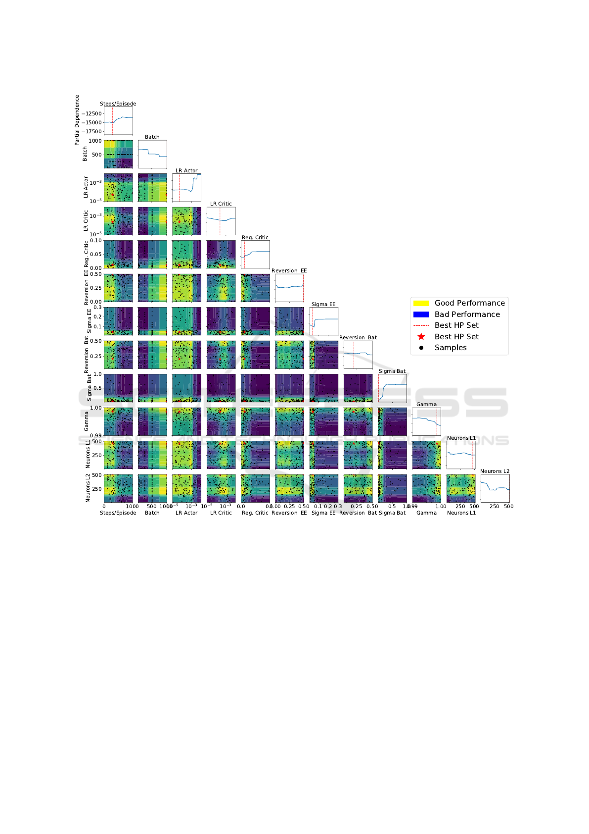
Figure 4: Sensitivity analysis of the hyperparameters. The ﬁgure shows the surrogate model of the hyperparameter optimiza-

tion for the entire hyperparameter space. It shows the individual samples, the sensitivities of the hyperparameters and the

interactions of the hyperparameters. Each row and column describes one hyperparameter. The sensitivity of the individual

hyperparameter is plotted in the diagonal. Relatively ﬂat curves as in Reversion Bat indicate that the hyperparameter is less

sensitive. In contrast, the curves of Sigma Bat and LR Actor indicate a more distinctive sensitivity. For the selection of the

best hyperparameters, the appropriate minima are of interest.

REFERENCES

Barsce, J. C., Palombarini, J. A., and Mart

ınez, E. C.

(2018). Towards autonomous reinforcement learning:

Automatic setting of hyper-parameters using bayesian

optimization. CoRR, abs/1805.04748.

Bergstra, J. and Bengio, Y. (2012). Random search for

hyper-parameter optimization. J. Mach. Learn. Res.,

13:281–305.

Breiman, L. (2001). Random forests. Machine Learning.

Brochu, E., Cora, V. M., and de Freitas, N. (2010). A

tutorial on bayesian optimization of expensive cost

functions, with application to active user model-

ing and hierarchical reinforcement learning. CoRR,

abs/1012.2599.

Chollet, F. (2017). Deep Learning with Python. Manning

Publications Co., Greenwich, CT, USA, 1st edition.

Duan, Y., Chen, X., Houthooft, R., Schulman, J., and

Abbeel, P. (2016). Benchmarking deep reinforcement

learning for continuous control. In Proceedings of the

33rd International Conference on International Con-

Hyperparameter Optimization for Deep Reinforcement Learning in Vehicle Energy Management

143

ference on Machine Learning - Volume 48, ICML’16,

pages 1329–1338. JMLR.org.

Falkner, S., Klein, A., and Hutter, F. (2018). Bohb: Robust

and efﬁcient hyperparameter optimization at scale. In

Proceedings of the 35rd International Conference on

International Conference on Machine Learning.

Graves, A., Mohamed, A., and Hinton, G. E. (2013).

Speech recognition with deep recurrent neural net-

works. CoRR, abs/1303.5778.

Henderson, P., Islam, R., Bachman, P., Pineau, J., Precup,

D., and Meger, D. (2017). Deep reinforcement learn-

ing that matters. CoRR, abs/1709.06560.

Hutter, F., Hoos, H. H., and Leyton-Brown, K. (2011). Se-

quential model-based optimization for general algo-

rithm conﬁguration.

Jones, D. R. (2001). A taxonomy of global optimiza-

tion methods based on response surfaces. Journal of

Global Optimization, 21(4):345–383.

Krizhevsky, A., Sutskever, I., and Hinton, G. E. (2012). Im-

agenet classiﬁcation with deep convolutional neural

networks. In Proceedings of the 25th International

Conference on Neural Information Processing Sys-

tems - Volume 1, NIPS’12, pages 1097–1105, USA.

Curran Associates Inc.

Liessner, R., Dietermann, A., B

aker, B., and L

upkes, K.

(2017). Generation of replacement vehicle speed cy-

cles based on extensive customer data by means of

markov models and threshold accepting. 6.

Liessner, R., Schroer, C., Dietermann, A., and B

aker, B.

(2018). Deep reinforcement learning for advanced

energy management of hybrid electric vehicles. In

Proceedings of the 10th International Conference on

Agents and Artiﬁcial Intelligence, ICAART 2018, Vol-

ume 2, Funchal, Madeira, Portugal, January 16-18,

2018., pages 61–72.

Lillicrap, T. P., Hunt, J. J., Pritzel, A., Heess, N., Erez, T.,

Tassa, Y., Silver, D., and Wierstra, D. (2015). Contin-

uous control with deep reinforcement learning. CoRR,

abs/1509.02971.

Lizotte, D. J. (2008). Practical Bayesian Optimization. PhD

thesis, Edmonton, Alta., Canada. AAINR46365.

Mania, H., Guy, A., and Recht, B. (2018). Simple random

search provides a competitive approach to reinforce-

ment learning. CoRR, abs/1803.07055.

Melis, G., Dyer, C., and Blunsom, P. (2017). On the state of

the art of evaluation in neural language models. CoRR,

abs/1707.05589.

Mnih, V., Kavukcuoglu, K., Silver, D., Rusu, A. A., Veness,

J., Bellemare, M. G., Graves, A., Riedmiller, M., Fid-

jeland, A. K., Ostrovski, G., et al. (2015). Human-

level control through deep reinforcement learning.

Nature, 518(7540):529.

Osborne, M., Garnett, R., and Roberts, S. (2009). Gaussian

processes for global optimization.

Plappert, M., Houthooft, R., Dhariwal, P., Sidor, S.,

Chen, R. Y., Chen, X., Asfour, T., Abbeel, P., and

Andrychowicz, M. (2017). Parameter space noise for

exploration. CoRR, abs/1706.01905.

Rupam Mahmood, A., Korenkevych, D., Vasan, G., Ma, W.,

and Bergstra, J. (2018). Benchmarking Reinforcement

Learning Algorithms on Real-World Robots. ArXiv e-

prints.

Shahriari, B., Swersky, K., Wang, Z., Adams, R. P., and

de Freitas, N. (2016). Taking the human out of the

loop: A review of bayesian optimization. In Proceed-

ings of the IEEE.

Silver, D., Schrittwieser, J., Simonyan, K., Antonoglou, I.,

Huang, A., Guez, A., Hubert, T., Baker, L., Lai, M.,

Bolton, A., et al. (2017). Mastering the game of go

without human knowledge. Nature, 550(7676):354.

Smith, S. L., Kindermans, P., and Le, Q. V. (2017). Don’t

decay the learning rate, increase the batch size. CoRR,

abs/1711.00489.

Snoek, J., Larochelle, H., and Adams, R. P. (2012). Prac-

tical bayesian optimization of machine learning algo-

rithms. In Pereira, F., Burges, C. J. C., Bottou, L., and

Weinberger, K. Q., editors, Advances in Neural In-

formation Processing Systems 25, pages 2951–2959.

Curran Associates, Inc.

Snoek, J., Rippel, O., Swersky, K., Satish, R. K. N., Sun-

daram, N., Patwary, M. M. A., Prabhat, and Adams,

R. P. (2015). Scalable bayesian optimization using

deep neural networks. In International Conference on

Machine Learning.

Springenberg, J. T., Klein, A., Falkner, S., and Hutter, F.

(2016). Bayesian optimization with robust bayesian

neural networks. In Proceedings of the 30th Interna-

tional Conference on Neural Information Processing

Systems, NIPS’16, pages 4141–4149, USA. Curran

Associates Inc.

Sutskever, I., Vinyals, O., and Le, Q. V. (2014). Sequence

to sequence learning with neural networks. CoRR,

abs/1409.3215.

Sutton, R. S. and Barto, A. G. (1998). Introduction to Re-

inforcement Learning. MIT Press, Cambridge, MA,

USA, 1st edition.

Sutton, R. S. and Barto, A. G. (2012). Reinforcement Learn-

ing: An Introduction. O’Reilly.

Thornton, C., Hutter, F., Hoos, H. H., and Leyton-Brown,

K. (2012). Auto-weka: Automated selection and

hyper-parameter optimization of classiﬁcation algo-

rithms. CoRR, abs/1208.3719.

Uhlenbeck, G. E. and Ornstein, L. S. (1930). On the theory

of the brownian motion. Phys. Rev., 36:823–841.

ICAART 2019 - 11th International Conference on Agents and Artiﬁcial Intelligence

144