Mixture of Multilayer Perceptron Regressions

Ryohei Nakano

and Seiya Satoh

Chubu University, 1200 Matsumoto-cho, Kasugai, 487-8501 Japan

Tokyo Denki University, Ishizaka, Hatoyama-machi, Hiki-gun, Saitama 350-0394 Japan

Keywords: Mixture Models, Regression, Multilayer Perceptrons, EM Algorithm, Model Selection.

Abstract:

This paper investigates mixture of multilayer perceptron (MLP) regressions. Although mixture of MLP re-

gressions (MoMR) can be a strong ﬁtting model for noisy data, the research on it has been rare. We employ

soft mixture approach and use the Expectation-Maximization (EM) algorithm as a basic learning method. Our

learning method goes in a double-looped manner; the outer loop is controlled by the EM and the inner loop

by MLP learning method. Given data, we will have many models; thus, we need a criterion to select the best.

Bayesian Information Criterion (BIC) is used here because it works nicely for MLP model selection. Our ex-

periments showed that the proposed MoMR method found the expected MoMR model as the best for artiﬁcial

data and selected the MoMR model having smaller error than any linear models for real noisy data.

1 INTRODUCTION

Mixture models have been widely used in economet-

rics, marketing, biology, chemistry, and many other

ﬁelds. The book by McLachlan and Peel (McLachlan

and Peel, 2000) contains a comprehensive review of

ﬁnite mixture models.

When data arise from heterogeneous contexts, it

is reasonable to introduce mixture of regressions as a

class of mixture models. In mixture of regressions,

since the introduction by Goldfeld and Quandt (Gold-

feld and Quandt, 1973), mixture of linear regres-

sions (MoLR) has been focused (Bishop, 2006; Qian

and Wu, 2011) and implemented as library programs

(Leisch, 2004; NCSS, 2013). Around that time,

Bayesian approaches to mixture of regressions were

vigorously investigated using Markov chain Monte

Carlo (MCMC) methods (Hurn et al., 2003).

Since this world is full of nonlinear relationships,

mixture of nonlinear regressions may have the great

potential. The research on the topic, however, has

been relatively few. Huang, Li, and Wang (Huang

et al., 2013) investigated mixture of nonlinear regres-

sions by employing kernel regression, but they as-

sumed that explanatory variable is univariate and the

extension to multivariate will suffer from curse of di-

mensionality; this can be a serious limitation.

As another approach, modal regression (Chen

et al., 2016) estimates the local modes of the distri-

bution of a dependent variable given a value of an ex-

planatory variable. Modal regression, however, will

not give us an explicit representation and the extend-

ability to multivariate data seems not clear.

Since multilayer perceptron (MLP) is a popular

powerful nonlinear model, mixture of MLP regres-

sions (MoMR) will be quite a reasonable model of

mixture of nonlinear regressions; however, MoMR

has hardly been addressed so far.

This paper investigates MoMR. There can be two

types of mixture: hard and soft. In hard mixture a data

point is exclusively classiﬁed, while in the latter a data

point belongs probabilistically to every class. Since

soft mixture is more natural for modeling and more

appropriate for computation, we employ soft mix-

ture approach, and use the Expectation-Maximization

(EM) algorithm (Dempster et al., 1977).

This paper is organized as follows. Section 2 re-

views the background of our research, and Section 3

explains modeling, EM solver, and model selection

of MoMR. Then Section 4 describes our experiments

performed to examine how our MoMR works using a

two-class artiﬁcial dataset and a noisy real dataset.

2 BACKGROUND

2.1 EM Algorithm

The EM algorithm is a general-purpose iterative algo-

rithm for maximum likelihood (ML) estimation in in-

Nakano, R. and Satoh, S.

Mixture of Multilayer Perceptron Regressions.

DOI: 10.5220/0007367405090516

In Proceedings of the 8th International Conference on Pattern Recognition Applications and Methods (ICPRAM 2019), pages 509-516

ISBN: 978-989-758-351-3

509

complete data problems (Dempster et al., 1977). The

EM and its variants have been applied in many appli-

cations (McLachlan and Peel, 2000).

Suppose that a data point (x,z) is generated with

the density p(x, z|θ), where only x is observable and z

is hidden. Here θ denotes a parameter vector, and let

p(x|θ) be the density generating x. In the EM context,

{(x

)} is called complete data, and {x

} is called

incomplete data, where µ = 1, ··· , N.

The purpose of ML estimation is to maximize the

following log-likelihood from incomplete data.

L(θ) =

∑

log p(x

|θ). (1)

The EM performs ML estimation by iteratively maxi-

mizing the following Q-function, where θ

(t)

is the es-

timate obtained after the t-th iteration.

Q(θ|θ

(t)

) =

∑

P(z

,θ

(t)

)log p(x

|θ), (2)

where P(z

,θ

(t)

) =

p(x

|θ

(t)

)

∑

p(x

|θ

(t)

)

. (3)

The EM algorithm goes as below.

[EM Algorithm]

1. Initialize θ

(0)

and t ← 0.

2. Iterate the following EM-step until convergence.

E-step: Compute Q(θ|θ

(t)

) by computing the

posterior P(z

,θ

(t)

M-step: θ

(t+1)

= argmax

Q(θ|θ

(t)

) and

t ←t + 1.

It can be shown that the EM iteration makes

the likelihood L(θ) increase monotonically; that is,

L(θ

(t+1)

) ≥ L(θ

(t)

), which means {θ

(t)

} converges to

a local maximum.

2.2 MLP Learning Methods

In this paper we employ three MLP learning methods

described below. Hereafter MLP(J) indicates MLP

having J hidden units and one output unit.

The BP algorithm (Rumelhart et al., 1986) is well-

known method of MLP learning. BP uses only the

gradient and goes in an online mode. BP is beautifully

simple and easily adaptable to many layers, used even

for deep learning (Goodfellow et al., 2016).

Although BP is widely used, its learning speed is

usually very slow and its capability to ﬁnd excellent

solutions is quite limited; thus, to accelerate the con-

vergence and improve the limited capability, several

methods were proposed (Luenberger, 1984). Here we

employ quasi-Newton method called BPQ (BP based

on quasi-Newton) (Saito and Nakano, 1997). BPQ

uses the Broyden-Fletcher-Goldfarb-Shanno (BFGS)

update to get a search direction, and uses 2nd-order

approximation to get a suitable step length. Getting a

suitable step length usually requires a lot of time, but

2nd-order approximation is carried out very quickly.

Recently, singularity stairs following (SSF) has

been proposed as a very powerful learning method of

single MLPs (Satoh and Nakano, 2013). SSF suc-

cessively learns MLPs to stably and systematically

ﬁnd excellent solutions, making good use of singu-

lar regions generated by using the optimal solution of

one-step smaller model MLP(J−1), and guaranteeing

monotonic decrease of training errors.

2.3 Model Selection

Since we consider many candidates of mixture mod-

els, we need a criterion to evaluate the desirability

of each candidate. For this purpose we make use

of information criterion, which indicates a trade-off

between learning error and model complexity. Al-

though many information criteria have been proposed

so far, we employ the Bayesian information criterion

BIC (Schwarz, 1978), because BIC stably showed

nice performance on MLP model selection (Satoh and

Nakano, 2017).

Let p(x|θ) be a learning model with parameter

vector θ. Given data {x

, µ = 1,···,N}, the log-

likelihood is deﬁned as shown in eq.(1) Let

θ be a

maximum likelihood estimate. BIC is obtained as an

estimator of free energy F(D) shown below, where

p(D) is called evidence and p(θ) is a prior of θ.

(

) =

−

log

(

)

(4)

p(D) =

∫

p(θ)

∏

µ=1

p(x

|θ) dθ (5)

BIC is derived using the asymptotic normality and

Laplace approximation.

BIC = −2L(

θ) + M logN

= −2

∑

log p(x

θ) + M logN (6)

BIC is calculated using only one point ML estimate

θ, where M is the number of parameters.

We consider another important measure for re-

gression: goodness of ﬁt. Total sum of squares (TSS)

indicates how much variation the data have, resid-

ual sum of squares (RSS) indicates the discrepancy

between the data and the estimates, and explained

sum of squares (ESS) indicates how well a regression

model represents the data. Given data {(x

),µ =

1,··· ,N}, TSS, RSS, and ESS are given as below,

where x are explanatory variables, y is a dependent

ICPRAM 2019 - 8th International Conference on Pattern Recognition Applications and Methods

510

variable, f

= f (x

) is an estimate obtained by a re-

gression function, and y

is a mean of

TSS =

∑

−y)

, RSS =

∑

( f

−y

)

(7)

ESS = T SS −RSS (8)

Thus, ESS/TSS (= 1−RSS/TSS) is an important mea-

sure indicating goodness of ﬁt of a regression model.

It is also called coefﬁcient of determination in the lin-

ear regression context.

3 MIXTURE OF MLP

REGRESSIONS

3.1 Modeling of MoMR

This subsection formalizes the MoMR model.

Let x = (x

,··· ,x

)

be K explanatory variables,

and y be a dependent variable. In this paper a

de-

notes the transpose of a.

Given data {(x

),µ = 1,··· ,N}, we consider a

mixture of C regression functions. Let f (x|w

) be a

regression function of class c(= 1,··· ,C), where w

is the weight vector. Since each regression function is

supposed to have a constant term, we extend a vector

of explanatory variables to get

x = (1,x

,··· ,x

)

MLP of class c has K input units, J

hidden units,

and one output unit. It also has weight vectors w

(c)

between all input units and hidden unit j(=1,··· ,J

and weights v

(c)

between hidden unit j(=0,1,··· , J

)

and an output unit. Then its regression function is

deﬁned as follows.

f (x|w

) = v

(c)

∑

j=1

(c)



(c)

)



(9)

Here w

= (v

(c)

,··· ,v

(c)

,(w

(c)

)

,··· ,(w

(c)

)

for c = 1, ··· ,C, and σ(h) denotes the sigmoid activa-

tion function. When J

= 1, we consider the following

linear regression function instead of MLP(J

=1).

f (x|w

) = w

x (10)

We assume the value of y is generated by adding a

noise ε

to a value of f (x|w

); here, ε

is supposed to

follow the Gaussian with mean 0 and variance σ

∼ N (0,σ

) (11)

Then, the dependent variable y follows the following

distribution.

y ∼ N ( f (x|w

), σ

) (12)

Let π

be the mixing coefﬁcient of class c. Then,

the density of complete data is described as follows.

p(y,c|θ

) = π

(y|f (x|w

),σ

) (13)

Here g(u|m,s

) denotes a density function where u

follows one-dimensional Gaussian with mean m and

variance s

g(u|m,s

) =

√

2π s

exp



−

(u −m)

2 s



(14)

The density of incomplete data is written as follows.

p(y|θ) =

∑

c=1

p(y,c|θ

) =

∑

(y|f (x|w

),σ

) (15)

Here θ is a vector comprised of all parameters, where

is a parameter vector of class c.

θ = (θ

,··· ,θ

)

, θ

= (π

, w

, σ

)

(16)

3.2 EM Solver of MoMR

Bishop describes the framework to solve soft mix-

ture of linear regressions (Bishop, 2006). We extend

Bishop’s framework to solve soft mixture of nonlinear

regressions, including MoMR.

Since class c is a latent variable and cannot be ob-

served, we employ the EM algorithm as a basic learn-

ing method to solve the problem.

Posterior probability P(c|y,θ) indicates the proba-

bility that y belongs to class c under θ.

P(c|y,θ) =

p(y,c|θ)

∑

p(y,c|θ)

(17)

Given data D = {(x

),µ = 1,··· ,N}, the log-

likelihood is deﬁned as below.

L(θ) =

∑

µ=1

log p(y

|θ) (18)

The Q-function to maximize is shown as below.

Here θ

(t)

denotes the estimate obtained at the t-th step

of the EM, and let f

≡ f (x

Q(θ|θ

(t)

) =

∑

µ=1

∑

c=1

P(c|y

,θ

(t)

) log p(y

,c|θ)

∑

µ(t)

log(π

,σ

))

∑

µ(t)



logπ

−

log(2π)

−log σ

−

− f

)

2σ



(19)

Mixture of Multilayer Perceptron Regressions

511

In the above, we use the following for brevity.

µ(t)

≡ P(c|y

,θ

(t)

) =

(t)

µ(t)

∑

(t)

µ(t)

(20)

where g

µ(t)

≡ g

µ(t)

,σ

2(t)

) (21)

When we maximize the Q-function, we use the La-

grange method since there is an equality constraint

∑

= 1. The Lagrangian function can be written as

follows with λ as a Lagrange multiplier.

J = Q(θ|θ

(t)

) −λ



∑

−1



(22)

The necessary condition for a local maximizer is

shown below for c = 1, ··· ,C.

∂J

∂π

∑

µ(t)

/π

−λ = 0 (23)

∂J

∂w

∑

µ(t)

− f

)

∂ f

∂w

= 0 (24)

∂J

∂σ

∑

µ(t)



−

− f

)



=0 (25)

Since we have λ = N from eq.(23) and the equality

constraint, a new estimate of π

is given below.

(t+1)

∑

µ(t)

(26)

From eq.(25) a new estimate of σ

is given below.

(σ

)

(

)

∑

µ(t)

− f

)

∑

µ(t)

(27)

From eq.(24) we obtain a new estimate of w

solving the following.

∑

µ(t)

− f

)

∂ f

∂w

= 0 (28)

Note that the condition eq.(28) is equal to the follow-

ing optimal condition of E

∂E

)

∂w

= 0. (29)

Here the following is sum-of-squares error of class c.

) =

∑

µ(t)

( f

−y

)

(30)

Residual sum of squares (RSS) in MoMR is given as

below.

RSS = 2

∑

) =

∑

µ(t)

( f

−y

)

(31)

In E

), squared error ( f

−y

)

for data point µ

is weighted by posterior P

µ(t)

. Thus, in MLP learn-

ing of class c, the gradient for data point µ should be

weighted by posterior P

µ(t)

. This modiﬁcation should

be embodied in MLP learning methods.

The learning of MoMR is carried out in a double-

looped manner: the outer loop is controlled by the EM

and the inner loop is controlled by MLP learning BP

or BPQ.

3.3 Model Selection of MoMR

This subsection describes how BIC is calculated in

MoMR.

The density of incomplete data is given by eq.(15).

Then, log-likelihood at the optimal point

θ is given as

follows.

(

) =

∑

µ=1

log p(y

θ)

∑

log



∑

|f (x

)



(32)

Hence, BIC in MoMR is obtained as below.

BIC = −2

∑

log



∑

g(y

|f (x

)



+ M log N (33)

Here M, the number of parameters, is calculated as

follows. We should not forget to count two parame-

ters π

and σ

in calculating M

M =

∑

, M



K + 3 if J

= 1

(K + 2)+ 3 if J

≥ 2

(34)

TSS, RSS and ESS in MoMR are shown below,

where each data point µ is weighted by posterior P

µ(t)

TSS =

∑

µ(t)

−y)

(35)

RSS =

∑

µ(t)

( f

−y

)

(36)

ESS = T SS −RSS (37)

Goodness of ﬁt ESS/TSS in MoMR is calculated us-

ing the above.

4 EXPERIMENTS

4.1 Design of Experiments

The following 26 models are considered for each

dataset. Models are given numbers, which are used

in the ﬁgures and explanations shown later.

ICPRAM 2019 - 8th International Conference on Pattern Recognition Applications and Methods

512

(a) Models 1 to 10: 10 single MLP(J) regressions:

J = 1,··· ,10,

(b) Models 11 to 16: 6 mixtures of MLP( J

) and

MLP(J

) regressions: (J

) = (1,1), (1,2), (1,3),

(2,2), (2,3), (3,3),

MLP(J

) and MLP(J

) regressions: (J

) =

(1,1,1), (1,1,2), (1,1,3),(1,2,2), (1,2,3), (1,3,3),

(2,2,2), (2,2,3), (2,3,3), (3,3,3).

Note that MLP( J=1) is replaced with linear regres-

sion here. Thus, Model 1 is a simple linear regres-

sion, Model 11 is a mixture of two linear regressions,

and Model 17 is a mixture of three linear regressions.

Model 12 is a mixture of one linear regression and one

MLP(J=2), and so on. As for the learning of mixture

of linear regressions (MoLR), refer to (Nakano and

Satoh, 2018). A single MLP(J) regression is learned

by SSF or BP if J ≥ 2.

Parameters of BP and BPQ are selected through

our preliminary experiments, as shown in Table 1.

Very weak regularization of weight decay is em-

ployed to prevent weight values from getting huge.

Note that the maximum of sweeps per EM loop needs

not be large since posterior may change during EM

learning. For SSF, maximum of search tokens is set

to be 20. We used a PC with Xeon(R)E5 3.7GHz with

8GB memory for computation.

Table 1: Learning parameters for the experiments.

Parameter BP BPQ

max sweeps/EM loop (MoMR) 500 500

learning rate (MoMR) 0.05 adaptive

weight decay coeff (MoMR) 10

−7

−6

max sweeps (Single) 5000 5000

learning rate (Single) 0.05 adaptive

weight decay coeff (Single) 10

−7

−6

4.2 Experiments using Artiﬁcial Data

We generated one-dimensional 2 class artiﬁcial data.

The following two parabolas were used to generate 51

data points for each class by adding Gaussian noise

N (0,0.035

). The range of x

is [0.1, 1.0].

= −4(x

−0.6)

+ 2.0 (38)

= −2(x

−0.6)

+ 1.5 (39)

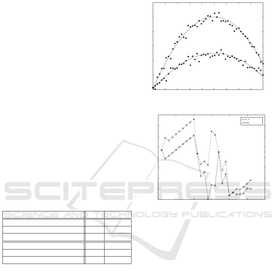
Figure 1 shows two parabolas and 102 data points.

Since MLP(J ≥ 2) can ﬁt a parabola well, two

MLPs(J=2) are expected to ﬁt this artiﬁcial data well

as the minimal model.

Figure 2 compares BIC of each model for artiﬁcial

data. Horizontal axis indicates model number.

0.1 0.2 0.3 0.4 0.5 0.6 0.7 0.8 0.9 1

x axis

1.2

1.4

1.6

1.8

2.2

y axis

Figure 1: Artiﬁcial data with two generating parabolas.

0 5 10 15 20 25 30

Model number

-200

-150

-100

-50

100

150

200

BIC

EM+BP

EM+BPQ

Figure 2: BIC comparison for artiﬁcial data.

BIC obtained by EM+BPQ was always smaller

(better) than the corresponding BIC by EM+BP ex-

cept pure linear Models 1, 11 and 17. This was caused

by BP’s weak capability to ﬁnd excellent solutions.

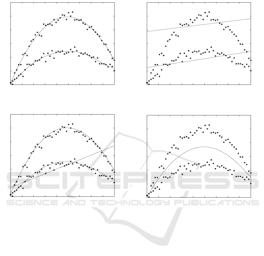
BIC obtained by EM+BPQ selected Model 14,

two MLPs(J=2), as the best among all the models,

which we expected. Figure 3 depicts Model 14. We

can see these two curves are very close to the original

parabolas.

BIC obtained by EM+BP selected Model 20, one

linear and two MLPs(J=2), as the best, whose BIC is

larger than Model 14. Figure 4 shows Model 20.

As the best mixture of linear regressions, BIC se-

lected Model 11, which is composed of two lines.

Figure 5 depicts Model 11. Its BIC was larger (worse)

than that of the best single MLP model (Model 2),

Among single regression models, BIC obtained

by SSF selected Model 2, MLP(J=2), while BIC ob-

tained by BP selected wrong Model 1, linear regres-

sion. Figure 6 shows Model 2, which runs in a middle

empty space between two parabolas.

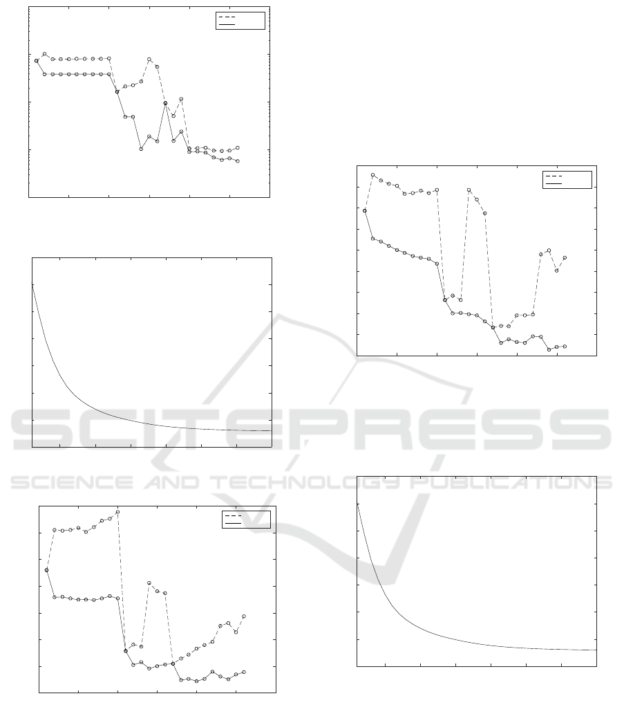
Figure 7 compares residual sum of squares (RSS)

of each model for artiﬁcial data. It can be seen that the

Mixture of Multilayer Perceptron Regressions

513

0.1 0.2 0.3 0.4 0.5 0.6 0.7 0.8 0.9 1

x axis

1.2

1.4

1.6

1.8

2.2

y axis

Figure 3: Best MoMR model obtained by EM+BPQ for ar-

tiﬁcial data.

0.1 0.2 0.3 0.4 0.5 0.6 0.7 0.8 0.9 1

x axis

1.2

1.4

1.6

1.8

2.2

y axis

Figure 4: Best MoMR model obtained by EM+BP for arti-

ﬁcial data.

solid line (EM+BPQ) always indicates smaller RSS

than the dotted line (EM+BP) except pure linear Mod-

els 1, 11 and 17. RSS of Model 14, the best model ob-

tained by EM+BPQ, was 0.1046 and thus its goodness

of ﬁt 1−RSS/TSS was very high 0.9867 since TSS =

7.8436 for artiﬁcial data. Moreover, the solid line in-

dicates that mixture models achieved much smaller

RSS than single models. Among mixture models, the

solid line also indicates that MoMR models had much

smaller RSS than mixture of pure linear regressions,

Models 11 and 17. Hence we can say MoMR effec-

tively improved goodness of ﬁt compared with single

regression models or mixtures of linear regressions.

Figure 8 indicates how RSS decreased through

EM learning in the best Model 14. The error de-

creased very smoothly and monotonically.

The CPU time required to get the results for arti-

ﬁcial data is compared below. As average CPU time

required to learn 16 MoMR models per initialization,

EM+BPQ required 1m 12s, while EM+BP required

7m 16s. Although BPQ computes more information

0.1 0.2 0.3 0.4 0.5 0.6 0.7 0.8 0.9 1

x axis

1.2

1.4

1.6

1.8

2.2

y axis

Figure 5: Best mixture of linear regressions for artiﬁcial

data.

0.1 0.2 0.3 0.4 0.5 0.6 0.7 0.8 0.9 1

x axis

1.2

1.4

1.6

1.8

2.2

y axis

Figure 6: Best single regression for artiﬁcial data.

than BP, its average CPU time was smaller because it

converged faster for this dataset.

4.3 Experiments using Real Data

As real data we used Abalone dataset from UCI Ma-

chine Learning Repository. We selected this dataset

because any single powerful regression model cannot

ﬁt well. The dataset has seven numerical explanatory

variables and the number of data points N = 4177.

Figure 9 compares BIC of each model for Abalone

data. It can be seen that BIC obtained by EM+BPQ

was always much smaller (better) than the corre-

sponding BIC by EM+BP except three pure lin-

ear models. BIC(EM+BPQ) selected Model 20,

one linear and two MLPs(J=2), as the best, while

BIC(EM+BP) selected inadequate Model 17, mixture

of two linear regressions, as the best. Note that Model

20 had smaller BIC than any single model or any

mixture of linear regressions. Among single models

MLP(J=7) is the best single model.

ICPRAM 2019 - 8th International Conference on Pattern Recognition Applications and Methods

514

0 5 10 15 20 25 30

Model number

-2

-1

RSS

EM+BP

EM+BPQ

Figure 7: RSS comparison for artiﬁcial data.

5 10 15 20 25 30 35

EM loops

600

800

1000

1200

1400

1600

1800

2000

RSS

Figure 8: EM learning of best Model 14 for artiﬁcial data.

0 5 10 15 20 25 30

Model number

6500

7000

7500

8000

8500

9000

9500

10000

BIC

EM+BP

EM+BPQ

Figure 9: BIC comparison for Abalone data.

Figure 10 compares RSS of each model for

Abalone data. We can see that EM+BPQ always

obtained much smaller RSS than EM+BP except

three linear models. RSS of the best single model

MLP(J=7) was 1543.36, then the goodness of ﬁt, co-

efﬁcient of determination, was 1−RSS/TSS = 0.6304,

which is not so high. Note that TSS = 4176 for nor-

malized Abalone data. RSS of Model 20, the best

model among all the models obtained by EM+BPQ,

was 727.32, then the goodness of ﬁt was 1−RSS/TSS

= 0.8258, showing nice ﬁtting. RSS of Model 17, the

best mixture of linear regressions, was 865.32, and its

goodness of ﬁt was 0.7928, a bit worse than the best

model. Model 24 had the smallest RSS 656.00 among

all the models, and its goodness of ﬁt was 0.8429.

Goodness of ﬁt for Abalone data can be improved to

this level by using MoMR.

0 5 10 15 20 25 30

Model number

600

800

1000

1200

1400

1600

1800

2000

2200

2400

RSS

EM+BP

EM+BPQ

Figure 10: RSS comparison for Abalone data.

Figure 11 indicates how RSS decreased through

EM learning in the best Model 20. The error de-

creased very smoothly and monotonically.

5 10 15 20 25 30 35

EM loops

600

800

1000

1200

1400

1600

1800

2000

RSS

Figure 11: EM learning of best model for Abalone data.

The CPU time required to get the results for

Abalone data is shown here. As average CPU time

required to learn 16 MoMR models per initializa-

tion, EM+BPQ required 6h 7m 40s, while EM+BP

required 4h 46m 37s.

4.4 Considerations

The experimental results may suggest the following.

Mixture of Multilayer Perceptron Regressions

515

(a) MoMR worked well, selecting the expected model

MLPs(J = 2) as the best for artiﬁcial data, and select-

ing the model composed of one linear and two MLPs

as the best for Abalone data. These best models show

smaller BIC and RSS values than those of any mixture

of linear regressions or any single MLP regression.

(b) The learning of MoMR goes in a double loop;

the EM controls the outer loop and MLP learning

method controls the inner loop. As for MLP learning,

a quasi-Newton method called BPQ worked well for

MoMR, while BP worked rather poorly, frequently

ﬁnding rather poor solutions, having larger (worse)

RSS than BPQ, selecting inadequate models differ-

ent from those by BPQ. This tendency was caused by

BP’s weak capability to ﬁnd excellent solutions.

goodness of ﬁt for data having poor ﬁt by any single

regression model or mixture of linear regressions.

5 CONCLUSIONS

This paper proposes modeling and learning of mix-

ture of MLP regressions (MoMR). The learning of

MoMR goes in a double loop; the outer loop is con-

trolled by the EM and the inner by MLP learning. As

for MLP learning in MoMR, a quasi-Newton worked

satisfactorily, while BP did not work. Our experi-

ments showed MoMR worked well for artiﬁcial and

real datasets. In the future we plan to apply MoMR

using EM+BPQ to more data to show MoMR can be

a useful regression model for noisy data.

ACKNOWLEDGMENT

This work was supported by Grants-in-Aid for Scien-

tiﬁc Research (C) 16K00342.

REFERENCES

Bishop, C. M. (2006). Pattern recognition and machine

learning. Springer.

Chen, Y.-C., Genovese, C., Tibshirani, R., and Wasserman,

L. (2016). Nonparametric modal regression. The An-

nals of Statistics, 44(2):489–514.

Dempster, A. P., Laird, N. M., and Rubin, D. B. (1977).

Maximum-likelihood from incomplete data via the

EM algorithm. J. Royal Statist. Soc. Ser. B, 39:1–38.

Goldfeld, S. and Quandt, R. (1973). A Markov model

for switching regressions. Journal of Econometrics,

1(1):3–15.

Goodfellow, I., Bengio, Y., and Courville, A. (2016). Deep

learning. MIT Press.

Huang, M., Runze, L., and Shaoli, W. (2013). Nonpara-

metric mixture of regression models. Journal of the

American Association, 108(503):929–941.

Hurn, M., Justel, A., and Robert, C. (2003). Estimating

mixtures of regressions. Journal of Computational

and Graphical Statistics, 12(1):1–25.

Leisch, F. (2004). FlexMix: A general framework for ﬁ-

nite mixture models and latent class regression in R.

Journal of Statistical Software, 11(8):1–18.

Luenberger, D. G. (1984). Linear and nonlinear program-

ming. Addison-Wesley.

McLachlan, G. J. and Peel, D. (2000). Finite mixture mod-

els. John Wiley & Sons.

Nakano, R. and Satoh, S. (2018). Weak dependence on ini-

tialization in mixture of linear regressions. In Proc. of

Int. Conf. on Artiﬁcial Intelligence and Applications

2018, pages 1–6.

NCSS (2013). Regression clustering. Technical Report

Chapter 449, pp.1–7, NCSS Statistical Software Doc-

umentation.

Qian, G. and Wu, Y. (2011). Estimation and selection in

regression clustering. European Journal of Pure and

Applied Mathematics, 4(4):455–466.

Rumelhart, D. E., Hinton, G. E., and Williams, R. J. (1986).

Learning internal representations by error propaga-

tion. In Parallel Distributed Processing, Vol.1, pages

318–362. MIT Press.

Saito, K. and Nakano, R. (1997). Partial BFGS update and

efﬁcient step-length calculation for three-layer neural

networks. Neural Comput., 9(1):239–257.

Satoh, S. and Nakano, R. (2013). Fast and stable learn-

ing utilizing singular regions of multilayer perceptron.

Neural Processing Letters, 38(2):99–115.

Satoh, S. and Nakano, R. (2017). How new information

criteria WAIC and WBIC worked for MLP model se-

lection. In Proc. of 6th Int. Conf. on Pattern Recog-

nition Applications and Methods (ICPRAM), pages

105–111.

Schwarz, G. (1978). Estimating the dimension of a model.

Annals of Statistics, 6:461–464.

ICPRAM 2019 - 8th International Conference on Pattern Recognition Applications and Methods

516