Detecting Adversarial Examples in Deep Neural Networks using
Normalizing Filters
Shuangchi Gu
1
, Ping Yi
1
, Ting Zhu
2
, Yao Yao
2
and Wei Wang
2
1
School of Cyber Security, Shanghai Jiao Tong University, 800 Dongchuan Road, Shanghai, China
2
Department of Computer Science and Electrical Engineering, University of Maryland Baltimore County, Baltimore, U.S.A.
Keywords:
Normalizing Filter, Adversarial Example, Detection Framework.
Abstract:
Deep neural networks are vulnerable to adversarial examples which are inputs modified with unnoticeable
but malicious perturbations. Most defending methods only focus on tuning the DNN itself, but we propose
a novel defending method which modifies the input data to detect the adversarial examples. We establish a
detection framework based on normalizing filters that can partially erase those perturbations by smoothing the
input image or depth reduction work. The framework gives the decision by comparing the classification results
of original input and multiple normalized inputs. Using several combinations of gaussian blur filter, median
blur filter and depth reduction filter, the evaluation results reaches a high detection rate and achieves partial
restoration work of adversarial examples in MNIST dataset. The whole detection framework is a low-cost
highly extensible strategy in DNN defending works.
1 INTRODUCTION
Deep learning technology is being widely used in
many industry fields, and Deep Neural Networks per-
form especially well on some artificial intelligence
tasks. For instance, researchers use DNNs to clas-
sify images, sounds, and texts. In some specific sit-
uations like security applications, the robustness of
the DNNs is important. However, recent studies have
shown that DNN attackers can modify some images
to misdirect the Deep Learning classification models,
forcing them to misclassify those images. The ma-
liciously generated images or other inputs are called
adversarial examples (Goodfellow et al., 2014).
Adversarial examples are normally crafted by
some specific attack algorithms. The hackers use such
algorithms to add small but effective perturbations to
contaminate the legitimate examples. The perturba-
tions are generally invisible to human eyes, but the
DNNs are susceptible to them. Basically, the exis-
tence of adversarial examples exposes the blind spots
in the DNNs’ training procedure.
The main goal of our work is to strengthen Deep
Neural Networks against the adversarial examples. A
pre-input framework is established to detect the ad-
versarial examples and transform some of those im-
ages to normal ones. The ability of detecting ad-
versarial examples is significant because even some
state-of-the-art DNN models are vulnerable to adver-
sarial attacks (Goodfellow et al., 2014), which means
that some DNN classifiers deployed online are hope-
less against those threats. That situation could be
changed with deploying a detecting method for the
input of DNNs.
Many previous works to strengthen the DNNs
have made some achievements. For instance, adver-
sarial training (Tram
`
er et al., 2017a) uses a large num-
ber of adversarial examples to retrain the DNN model.
It mainly focuses on modifying the model itself, and
the model would be able to defend one specific at-
tack after training with adversarial examples crafted
by that. Like adversarial training, many previous de-
fensive works could not defend several attack simul-
taneously, and cost a lot.
In a CNN classification system, the input is nor-
mally an 8bit grey image or a 24bit color image,
which means that the feature space of the input is un-
necessarily large. The training data is only a minor
part of the feature space, and the rest of the input
feature space will provide extensive probability for
the existence of adversarial examples. On the other
hand, the adversarial perturbations are mostly a mi-
nor modification on the legitimate image, so the dis-
tance between the legitimate and adversarial images
are relatively small. If some normalizing image fil-
ters are applied to the adversarial examples, the nega-
164
Gu, S., Yi, P., Zhu, T., Yao, Y. and Wang, W.
Detecting Adversarial Examples in Deep Neural Networks using Normalizing Filters.
DOI: 10.5220/0007370301640173
In Proceedings of the 11th International Conference on Agents and Artificial Intelligence (ICAART 2019), pages 164-173
ISBN: 978-989-758-350-6
Copyright
c
 2019 by SCITEPRESS – Science and Technology Publications, Lda. All rights reserved

tive effects of adversarial perturbations may be easily
erased. Based on that facts, the major contribution of
this paper is as follow.
• Low-cost filters based on normalizing algorithms
which can decrease the effect of adversarial per-
turbations are applied to the input images.
• We raised a novel normalized prediction inconsis-
tency algorithm which use the prediction vectors
to detect the adversarial examples.
• The pre-input framework based on normalizing
filters appears to be an effective and a less expen-
sive way to enhance the robustness of DNN mod-
els in our evaluation.
The paper is structured as follows. Section 2 in-
troduces basic technology about adversarial examples
and some previous work to defend adversarial attacks.
Several normalizing filters are presented in section 3
and will be evaluated with the framework in section
4.
2 BACKGROUND AND RELATED
WORKS
This section provides a concise introduction to adver-
sarial examples generating methods and normal de-
fensive methods.
2.1 Adversarial Examples Generating
Methods
An adversarial example is an input which is able to
mislead the target classifier but is not sensitive to hu-
man perception. It is crafted from a legitimate exam-
ple by an adversary with a limited perturbation.
Adversarial examples can be targeted, the legit-
imate example x would be classified as a particular
class by adversarial perturbation, formally, using a
given x ∈ X and classify function f (·), the goal of a
targeted adversarial attack with target α ∈ A is to find
an x
0
∈ X that
f

x
0

= α ∧ 4

x, x
0

≤ ε (1)
the 4 presents the distance between x and x
0
. Fur-
thermore, adversarial examples can be untargeted, in
which case the adversary’s goal is just for x
0
to be clas-
sified as any class other than its correct class, which
is
f

x
0

6= f (x) ∧ 4

x, x
0

≤ ε (2)
The perturbation intensity ε is the limit of image
modifications. The smaller it is, the more similar
the adversarial and legitimate examples are. In other
words, the adversarial example seems to be “legiti-
mate” to a human observer. In equation (1) and (2),
the distance function 4(x, x
0
) is basically a L
p
-norm
metric.
2.1.1 Fast Gradient Sign Method
Goodfellow et al. (Goodfellow et al., 2014) proposed
the fast gradient sign method (FGSM) to find the ad-
versarial examples effectively. The perturbation is
calculated directly by using gradient vector of the loss
function J (·, ·, ·) for training the target classifier:
η = εsign(∇
x
J (θ, x, f (x))) (3)
The adversarial examples processed by FGSM are
untargeted, and the perturbations are calculated using
the L
∞
-norm.
2.1.2 Basic Iterative Method
Kurakin et al. (Kurakin et al., 2016) raised the basic
iterative method (BIM) which is based on FGSM. The
adversarial applies FGSM multiple times with small
steps. For the original input x, the image at k iteration
is
x
0
k
= x
0
k−1
+Clip
x,ε

α · sign

∇
x
J

g

x
0
k−1

, y

(4)
The average distance between the legitimate and
adversarial examples in BIM method is smaller than
FGSM, which means the perturbations are harder to
detect by human perception.
2.1.3 Jacobian Saliency Map Approach
Jacobian saliency map approach (JSMA) is proposed
by Papernot et al. (Papernot et al., 2016c) which is a
targeted method with the perturbations limited by L
0
-
norm, so this attack only modify a limited pixels of
the original image. JSMA iteratively perturbs pixels
in an input image that have high adversarial saliency
scores. The adversarial saliency score of each pixel is
calculated to reflect how this pixel will increase pre-
diction probability of the target class α in the classi-
fier model while decrease the probability of all other
possible classes.
2.1.4 Carlini & Wagner Attack Method
Carlini et al. (Carlini and Wagner, 2017) recently in-
troduced a gradient-based attack which can generate
adversarial examples based on L
0
, L2, L
∞
-norms, and
it is more effective and stronger than other methods
introduced above.
The C&W attack will be the key generating
method in the evaluation section.
Detecting Adversarial Examples in Deep Neural Networks using Normalizing Filters
165

2.2 Defensive Methods against
Adversaries
The defensive methods could be divided into two
themes: model modification and data modification.
The former methods include adversarial training,
gradient masking (Papernot et al., 2016b) and oth-
ers which mainly focus on the optimization of the
CNN models. Adversarial training uses the adver-
sarial examples and their corresponding ground truth
labels as extra training data, thus the classifier would
learn how to avoid the negative influence of the ad-
versarial perturbations and become more robust ide-
ally. Gradient masking aims to reduce the sensitiv-
ity of the classifiers to minor changes in input images.
(Papernot et al., 2015) introduced a defensive distil-
lation strategy to hide the gradient information from
an adversary. But it was proved being vulnerable to
black-box attack. The input normalizing framework
proposed by us is a part of data modification, it keeps
the CNN models unchanged and uses different nor-
malizing filters to erase the minor perturbations.
As for detection, (Ma et al., 2018) raised a de-
tection method using local intrinsic dimensionality
(LID). The LID values of adversarial and legitimate
examples are different so that the system can detect
the adversarial examples if the LID value is abnor-
mal. Ping et al. (YI Ping and Jianhua, 2018) surveyed
the adversarial attacks in artificial intelligence.
3 NORMALIZING FILTERS &
DETECTION METHOD
The system structure of the whole framework is
shown in Fig. 1. In our work, we mainly focus on
filters which are able to decrease the redundant infor-
mation in the input images. After sufficient evalua-
tion on numbers of different digital filters, two types
of filters are deployed in Normalizing Filters Pack as
our “normalizing filters”: Gaussian & median blur fil-
ter and depth reduction filter, and the predictions of
images using different filters would be sent into the
judge module in Fig. 1, a proper algorithm based on
prediction inconsistency is applied to the module.
The framework has high flexibility. The CNN
classifier in the framework is replaceable. For each
classifier, a specific configuration would be set to fit
the input image type and format. The filters and
the detection algorithm for different prediction vec-
tors are also adjustable. Furthermore, the cost on the
whole system is relatively low, the requirements for a
long period of time and high-performance computa-
tion hardware is unnecessary.
3.1 Gaussian & Median Blur Filter
Blur filters are commonly used in daily situations
to reduce noise or hide some particular information,
which may be effective to “normalize” the perturba-
tions. Here we describe the two types of blur algo-
rithms.
3.1.1 Gaussian Blur Filter
The Gaussian blur filter uses a Gaussian function to
calculate the transformation to apply to each pixel in
the input image. With the standard deviation of the
Gaussian distribution σ set, a convolutional matrix
with dimensions
d
6σ
e
×
d
6σ
e
will be applied to the
original image (pixels at a distance of more than 3σ
have almost-zero influence). Applying a Gaussian fil-
ter with a proper deviation to an image does not mean
to lose key information in the original image, but can
partially remove the abruptly sharp pixels and edges,
which can be the consequences of adversarial pertur-
bations.
3.1.2 Median Blur Filter
The median blur filter’s theory is a resemblant of
Gaussian filter in image processing territory. The
main idea of the median filter is to run through the
original image pixel by pixel, replacing each pixel
with the median of neighboring ones. The filter cre-
ates a “slide window” which slides over the entire im-
age and finally output a smoothed image. The median
blur filter actually makes adjacent pixels more similar
and the slide window size is set according to differ-
ent adversarial attack types. For instance, a relatively
small value for window size will work on adversarial
perturbations calculated through L
0
-norm.
3.2 Depth Reduction Filter
Bit depth implies how redundant an image is in the
color or greyscale aspect. For most images in usual
cases, there would be some redundancy which means
the observer can reduce the bit depth while keeps the
key information in the original images. For instance,
a grayscale image in MNIST (LeCun et al., 1990)
provides 2
8
= 256 possible values for each pixel, but
the image actually keeps its information using 1-bit
depth filter. Thus, a depth reduction filter would not
evidently influence the target CNN classifier’s perfor-
mance.
For some attacks based on L
∞
-norm, the adversar-
ial perturbations appears to be fuzzy patterns, which
ICAART 2019 - 11th International Conference on Agents and Artificial Intelligence
166

Input
Image
Normalizing Filters Pack
filter 1 filter 2
filter 3 .........
CNN
Origin
Result
result 1
result 2
result 3
.......
Judge
F(conf,acc)
adv
yes/no
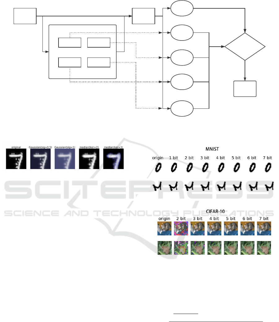
Figure 1: The Adversarial Examples Detection Framework. The CNN receives both original image and images modified by
normalizing filters, then the predictions are sent into judge module to figure out whether the original image is an adversarial.
Figure 2: Gaussian & median blur filters at multiple con-
figurations. Both filters are effective to reduce abruptly-
occurring pixels in this case.
indicates the color space of that image is too big to
generate a specific perturbation. Thus the adversarial
perturbations may be cleared if the color space is re-
duced. On the other hand, the bit depth should not be
too small if the image is relatively complicated, the
effect of different depth is shown in Fig. 3.
3.3 Implementations of Filters
The Gaussian and median blur filters we used in
the evaluation section are implemented in the Scipy
module (Jones et al., 2014). The median filter will
be set with a 2 × 2 slide window in low resolution
datasets and an additional 3 × 3 window in ImageNet
(Krizhevsky et al., 2012). case. As for Gaussian fil-
ters, different value of σ from 0.5 to 2.0 will be tested
in all datasets. Fig. 2 are living instance for both fil-
ters.
The formula below is adopted to simulate the
depth reduction filters. Variable ogdep and dep indi-
cate the bit depth of the original image (8 in the cho-
sen datasets) and the aim (1 to 7).
Figure 3: Depth Reduction Filters at different settings: as
shown in the MNIST dataset, the images still keep the
key information, but situations are totally opposite in the
CIFAR-10 dataset (Krizhevsky et al., 2014). As a result, the
depth reduction filter chosen in the final defensive frame-
work should be specified by the target CNN classifier.
rec =







img
2
ogdep
− 1
× 2
dep
− 1

× 2
ogdep
− 1
2
dep
− 1






(5)
3.4 Detection Methods
The basic method of detecting adversarial examples is
named prediction inconsistency (Hinton et al., 2012).
It means one adversarial example will have different
predictions using several classifiers which have the
Detecting Adversarial Examples in Deep Neural Networks using Normalizing Filters
167

same function.
However, (Tram
`
er et al., 2017b) have proved the
transferability of the adversarial examples even the
adversarial space, thus we raised a novel concept of
prediction inconsistency: normalized prediction in-
consistency. This method is based on the predictions
of the same image in several normalizing filters using
the same classifier. Because of the normalizing fil-
ters we use have little influence on legitimate exam-
ples, images which have the prediction inconsistency
issues are likely to be adversarial examples.
The methods to measure the distance between pre-
dictions is flexible. A prediction generated by the tar-
get classifier is represented as a vector of probabil-
ity distributions, thus, we can compare the vectors of
probability distributions using L
1
, L
2
-norms, or train-
ing a support vector machine to detect the normal-
ized prediction inconsistency phenomenon. We fi-
nally choose L
2
-norm-based distance to judge the dif-
ference in the evaluation section.
dist
(og, nmlzd)
2
=



f (x)
og
− f (x)
nmlzd



2
,
f (x) =
h
p
1
(x), p
2
(x), · · ·, p
k
(x)
i
(6)
Here f (x)
og
indicates the prediction vector of
original input image, and f (x)
nmlzd
is that of the im-
age “normalized” by one of the filters. Each predic-
tion vector should contain 5 to 10 probabilities in gen-
eral conditions.
Last but not the least, it is not enough to get the
distances between several prediction vectors, the al-
gorithm for calculating the inconsistency level and a
standard threshold value is significant for estimate the
comprehensive result whether the original input im-
age is adversarial. We noticed that different filters
have significantly different influence on the same ad-
versarial attack algorithm, so the larger the distance
is, the more important it could be.
f in
(k,dist)
2
=
1
n
∑
i
dist
k
i
, k = 1, 2, 3, · · · (7)
The parameter k here implies the importance of
outstandingly large distances, as k became bigger, the
value of dist
k
i
would tend to be zero if dist
i
is rela-
tively small, like distances in a legitimate example’s
case. Here parameter k would be 2 in our evaluation.
The normalizing filters and detecting methods fi-
nally just work together as Fig. 1.
4 EVALUATION OF
NORMALIZING FILTERS
After introduction about adversarial examples, nor-
malizing filters and detecting methods towards adver-
saries. We have arrived at some primary conclusion
and requirements:
• Many images used in the classification task con-
tain redundant and irrelevant information.
• Normalizing filters are designed to ignore the re-
dundancy of the input images.
• Normalizing filters should be able to destroy the
influence of adversarial perturbation.
• Normalizing filters should not impact the accu-
racy of the target CNN classifiers.
Next step is to evaluate whether normalizing fil-
ters could satisfy those requirements. In the next sec-
tion, the detecting methods will be tested combined
with filters.
4.1 Experiment Setup
The image classifiers we use are mentioned above:
Maxout Network (Goodfellow et al., 2013) for
MNIST provided by cleverhans (Papernot et al.,
2016a), DenseNet (Iandola et al., 2014) and
Inception-V3. The accuracy of the classifiers are
shown in Table 1.
Table 1: Statistics of Target CNN Classifiers.
Dataset & Classifier Top-1 Acc Top-5 Acc
MNIST Maxout Net 99.55% /
CIFAR-10 DenseNet 95.12% /
ILSVRC 12 Inception 78.8% 94.36%
The experiment contains up to seven attacks, in-
cluding targeted (CW @L
0
, CW @L
2
) and untargeted
attacks (FGSM, BIM, JSMA, CW @L
0
, CW @L
2
),
all of the implementations are provided by the clever-
hans lib (Papernot et al., 2016a). The hardware in the
experiment includes an Intel Xeon E5-2680 v3 CPU,
128GB DDR 4 ECC memory and an NVIDIA Tesla
M40 graphics card. For each dataset, we randomly
choose 500 legitimate images for each adversarial at-
tack, and we also adjust the parameters properly to
generate 1000 adversarial examples for each type of
attacks which have relatively high attack success rate
over 90% and short distance (L
0
, L
2
, L
∞
− norm) ac-
cording to the attack types, which is a guarantee for
a proper attack strength. The CW attack (Carlini and
ICAART 2019 - 11th International Conference on Agents and Artificial Intelligence
168

Wagner, 2017) could always generates adversarial ex-
amples with better attack success rate, and smaller
perturbations, but it just takes 10× more time to gen-
erate the perturbation.
As for targeted attacks, we used the least likely
class as the target, which has the smallest probability
in the prediction vector. Thus we have covered almost
all types of attacks in the evaluation.
4.2 Results on Normalizing Filters
The defence results are shown in Table 2 and some
are figured in Fig. 4. All of the seven attacks above
have been evaluated with three different datasets, and
three normalizing filters are tested with eight config-
urations.
Gaussian & Median Blur Filters. In theory, blur
algorithm would be effective to perturbations as
abruptly sharp pixels and edges because it basically
makes the pixels closer to their neighbors.
• MNIST. The gaussian and median filters both
have two configurations on MNIST datasets.
Both filters are relatively well performing against
JSMA and CW @L
0
attacks, which is close to
our hypothesis. As for the configurations, Gaus-
sian filters perform slightly better at σ = 0.6 than
σ = 0.4, and median filters perform worse at a
2 × 2 slide window than a 3 × 3 one. The effect
of both filters on MNIST images are quite close,
and the performance are similar too. It is note-
worthy that the blur filters have minor impact on
the accuracy of legitimate examples, which is par-
tially because the information of MNIST images
is quite simple and clear (just from 1 to 10).
• CIFAR-10. CIFAR-10 is basically a low reso-
lution color image dataset, which means the im-
ages look like “blurred”. So the configuration
should be set with discretion. The σ value of gaus-
sian filter is set to 0.3 which is lower than that
on MNIST images, the median filter just use the
smallest 2 × 2 slide window. For the results, the
performance is relatively satisfying on L
0
-norm
attacks which is close to the results on MNIST
dataset. The median filters work outstandingly
well against JSMA attacks, that may be a coin-
cidence because the limitation test batch size.
• ImageNet. The test results is slightly different on
ImageNet dataset. Firstly, we discover that both
filters have ordinary performance against FGSM
and BIM attacks which increase the classifying
accuracy up to 34.4%, it is an acceptable result for
L
∞
-norm attacks. Next, the performance on CW
L
0
and L
2
attacks are close (69.8% 81.2% by
median filter and 58.8% 70.6% by gaussian fil-
ter), that means the perturbation generated by CW
attack can be roughly erased by blur algorithms.
Actually, the truth is the perturbations of CW at-
tack are less sensitive to human perception, but
those tiny adjustment would be easily removed or
confused.
According to the statistics in the last column of
Table 2, the average confidence of normalized adver-
sarial examples (processed by gaussian and median
filters) decreases sharply, from about 90% to 60% in
MNIST and CIFAR-10, and from 80% to 50% in Im-
ageNet. That kind of decrease could be a signal of
prediction inconsistency phenomenon, which will be
discussed later.
Depth Reduction Filter. The major effect for depth
reduction filter is reducing the rebundancy in images.
The configuration of this filter varies in three datasets.
In MNIST, the depth is reduced to 1-bit, which means
it is actually a binary filter.In CIFAR-10 and Ima-
geNet, we use two configurations: 5-bit and 6-bit to
avoid losing the image’s major information.
• MNIST. The binary filter works properly against
L
∞
attacks. It boosts the accuracy to almost
100.0%, which is the same as legitimate exam-
ples’. The reason is obvious: the pixels in pertur-
bations calculated with L
∞
-norm are converted to
either 0 (white) or 1 (black), and in order to be in-
visible to human eyes, the value of each pixel is
always less than 0.5. The binary filter also out-
performs other defence strategy in Fig. 5 As for
CW @L
2
attack, the accuracy is still good at about
77.8%, but the binary filter seems to be in vain
against CW @L
0
attack.
• CIFAR-10. Results on 5-bit and 6-bit are nega-
tive. The prediction accuracy of normalized im-
age hardly reaches 30%, only the accuracy of CW
@L
2
attack cases reaches 48.2%, which still is not
a good result. The main reason of these results
comes from the format of the images, which is
32 × 32 24-bit color image, the resolution of each
sample is too low even human have to concentrate
to recognize it. Thus, we believe that the depth
reduction filter just simply ruins the image itself
but the perturbations.
• ImageNet. Depth reduction filter works unsatis-
fying against L
∞
andL
0
attacks on ImageNet ei-
ther. But the accuracy about L
2
attacks increases
to 56.4% (untargeted) and 50.3% (targeted). Like
what we have conclude above, the CW @L
2
attack
generates almost invisible perturbations which
can be easily influenced by other filters.
We have evaluated the performance of three filters
Detecting Adversarial Examples in Deep Neural Networks using Normalizing Filters
169

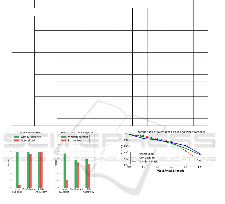
Table 2: Defence Statistics of Normalizing Filters: Pm. indicates the parameter of each filter, OAcc. is the accuracy of legiti-
mate examples using normalizing filters and Conf. is the average prediction confidence of normalized adversarial examples.
Type
Dataset Pm.
OAcc.
Accuracy Under Attacks
Conf.
FGSM BIM JSMA CW
0
CW
2
CW
0T
CW
2T
Gaussian
Filter
MNIST
0.4 99.2% 56.2% 28.6% 70.0% 50.2% 51.4% / / 60.5%
0.6 98.5% 49.8% 19.4% 80.8% 60.3% 66.8% / / 68.3%
CIFAR-10 0.3 88.3% 13.2% 15.2% 50.6% 70.6% 66.4% 68.8% 69.6% 72.1%
ImageNet
0.4 64.1% 34.4% 32.3% / 65.4% 58.8% 64.6% 59.0% 56.7%
0.6 62.8% 33.2% 29.8% / 70.6% 69.0% 66.6% 68.9% 60.6%
Median
Filter
MNIST
2x2 99.3% 60.2% 34.5% 70.2% 63.3% 43.2% / / 67.3%
3x3 99.0% 53.2% 20.3% 79.3% 60.4% 42.4% / / 64.3%
CIFAR-10 2x2 90.4% 40.4% 14.6% 90.8% 70.4% 56.2% 76.3% 60.2% 55.2%
ImageNet
2x2 66.5% 32.4% 33.2% / 69.8% 70.5% 81.2% 75.6% 50.3%
3x3 64.9% 32.8% 29.3% / 80.3% 68.4% 76.8% 79.0% 45.5%
Depth
Reduc-
tion
MNIST 1bit 99.3% 100% 99.2% 55.5% 5.4% 77.8% / / 93.8%
CIFAR-10
6bit 92.1% 20.8% 13.7% 12.4% 6.2% 39.1% 0.8% 48.2% 53.5%
5bit 93.4% 16.3% 10.6% 9.2% 10.1% 29.8% 1.6% 40.3% 46.1%
ImageNet
6bit 68.2% 9.8% 8.8% / 45.6% 56.4% 43.4% 50.3% 47.2%
5bit 70.4% 1.2% 0.2% / 22.1% 48.1% 19.8% 38.2% 43.5%
(a) Bit Depth @1bit (b) Median 3 × 3
Figure 4: Part of the normalizing results on three datasets.
The normalizing filters are effective to reduce the attack
strength while barely influence the accuracy on legitimate
examples.
so far. From the results in Table 2, it is obvious that
those filters are not strong enough to use as a stand-
alone defensive methods. However, some filters are
able to erase a specific type of perturbations and oth-
ers can reduce the confidence of adversarial examples,
in other words, the normalizing filters can either de-
stroy the perturbation or weaken it. Those features
are the headspring of the idea to develop a detection
framework using normalizing filters.
FGSM Attack Strength
Figure 5: The binary filters perform well comparing with
other defence methods. Here is the binary filter on MNIST
against FGSM at different attack strength, the binary filter
outperform the adversarial training and gradient masking at
a relatively low strength ε.
5 EVALUATION OF DETECTION
FRAMEWORK
The confidence data of section 4 has been collected to
analyze whether those adversarial examples have nor-
malized prediction inconsistency issues. Using equa-
tion (7), the f in
(2,dist)
2
values of both legitimate and
adversarial examples are shown in Fig. 6.
In Fig.6(a), most legitimate examples have no pre-
diction inconsistency issues, the peak is around 0, and
the situation is identical in Fig 6(b) with the peak
about 0.1. On the other hand adversarial examples
have an opposite circumstance, the peak is about 0.7
in MNIST and 0.6 in ImageNet.
ICAART 2019 - 11th International Conference on Agents and Artificial Intelligence
170

Table 3: Statistics of Detection Framework: The MNIST dataset has the best results for its high detection rate and low false
negative rate; Both CIFAR-10 and ImageNet are tested with two thresholds for either high detection rate or relatively low
FNR.
Dataset Configurations Thresholds Attacks Detection Rate FNR
MNIST
DRF 1-bit
Median 2x2
0.04
L
∞
97.43% 0.13%
L
2
98.20% 0%
L
0
95.61% 0.18%
CIFAR Median 2x2
0.221
L
∞
43.27% 1.42%
L
2
78.33% 1.04%
L
0
89.80% 0.41%
0.473
L
∞
28.72% 0.55%
L
2
66.07% 0.61%
L
0
74.48% 0.39%
ImageNet
Gaussian 0.6
Median 3x3
DRF 5-bit
0.342
L
∞
80.21% 0.52%
L
2
90.1% 0.41%
L
0
86.34% 0.42%
0.423
L
∞
77.54% 0.31%
L
2
87.2% 0.33%
L
0
84.32% 0.35%
Table 4: Comparison of the normalizing framework and the LID detecting method. The statistics are based on the result on
MNIST.
Methods Detect Rate FNR Cost Adaptability
Normalizing Framework 97.08% 0.10% Low High
LID 97.56% 0.13% Relatively High Medium
5.1 Detection Threshold
A detection threshold value for f in
(2,dist)
2
in equa-
tion (7) should be set. The threshold value would be
picked between two peaks in Fig. 6, and all images
that have higher f in
(2,dist)
2
value would be considered
as adversarial examples.
According to the results in Table 2, different
groups of normalizing filters are tested for the three
datasets, in MNIST, 1-bit depth reduction filter and
median filter with a 2 × 2 core are chosen in the de-
tection framework; we only use a median filter with a
2×2 core to normalize the CIFAR-10 images because
other filters have unsatisfying results; for ImageNet, a
gaussian filter with σ=0.6, a median filter with a 3 × 3
core, and a 5-bit depth reduction filter are chosen for
the test.
Table 3 represents the test results of thresholds,
which have been evaluated based on detection rate
and false negative rate (FNR). We use both 10,000 ad-
versarial and legitimate images for testing each con-
figuration, and 1000 images for CW@L
2
attacks of
ImageNet, which takes too much time.
• MNIST. Using 1-bit detph reduction filter and
median filter with 2 × 2 core, the detection frame-
work has a remarkable result on overall detection
rate of 97.08%, the score on L
0
, L
2
, L
∞
-norm at-
tacks are all satisfying with an acceptable false
negative rate at 0.103%. A lower threshold value
would have minor influence the detection rate
while significantly increase the false negative rate.
• CIFAR-10. Due to the unstable result on the
normalizing filters, there is only one filter used
in the CIFAR-10’s detection framework. The
biggest problem for other filters is the destruc-
tive modifications made to legitimate examples,
which causes the false negative rate unacceptable.
The results of the one-filter detection framework
is not bad. The detection rate for L
0
andL
2
attacks
reaches 78.33% and 89.80% with FNR at less than
1.10%. Although the detection rate of L
∞
attacks
are 43.27%, the legitimate examples are hardly
misjudged. A higher threshold at 0.473 can re-
duce the FNR to about 0.5%, but the detection rate
falls nearly 13.5%.
• ImageNet. Detection rate with threshold at 0.342
and 0.423 is both good with average scores at
Detecting Adversarial Examples in Deep Neural Networks using Normalizing Filters
171

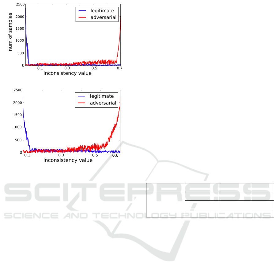
(a) MNIST inconsistency
(b) ImageNet inconsistency
Figure 6: The difference of prediction inconsistency phe-
nomenon between legitimate and adversarial examples, the
score is based on L
2
distance of the predictions of normal-
ized images and has a range from 0 to 1 in theory, but it
is almost impossible to reach the 1 value because the pre-
diction just varies after using the normalizing filters. The
MNIST case uses a binary filter and the ImageNet case uses
a median filter.
85.55% and 83.02%. But the difference in FNR
is attention-getting, the 0.423 threshold performs
way better than 0.342, especially in L
∞
attacks.
We suppose that is an accidental event in picking
test data.
Table 4 indicates the difference between the nor-
malizing detection framework and LID-based method
on MNIST dataset. We can conclude that the de-
tection rate and false negative rate are close, but for
the cost and adaptability of different CNN classifiers,
the normalizing detection framework performs better,
which is the main superiority. The LID method need
to analyze the inner structure of the neural network
and calculate the score at a deep layer of the classifier
to ensure the best performance, its adaptability is not
so good as the normalizing detection framework.
5.2 Restore Threshold
It is noticable that normalizing filters have impres-
sive performance in the MNIST dataset, and due
to adversarial perturbation is relatively unnoticeable
(small), most adversarial examples could be “normal-
ized” back to its original class, in other words, they
could be restored. Thus, a restore threshold could be
set to judge whether the prediction of adversarial ex-
ample after normalizing is the original class.
class
restore
=
h
class
p
, pred
p
i
,
pred
p
= max ( pred
1
, pred
2
, ·· · ) ,
pred
i
≥ th
restore
(8)
The restored class is calculated as equation (8),
here th
restore
is the restore threshold value. In the
prediction vector, only probabilities over the thresh-
old would be considered as a candidate. The test for
restore threshold value is in Table 5. As the data
indicates, higher threshold means better accuracy of
restoring, but fewer adversarial examples can be re-
stored, for instance, the accuracy at 0.9 threshold is
about 98.4% with a restored ratio at just 43.3%, but
the restore ratio at 0.750 threshold can reach 80.8%
with a lower restore accuracy.
Table 5: Restore Threshold and Restore Ratio for MNIST:
the input images are adversarial examples detected by our
detection framework. The threshold value is actually a re-
striction of confidence.
Env Threshold Accuracy RR
MNIST with
Detection
0.900 98.4% 43.3%
0.880 96.7% 56.2%
0.750 86.3% 80.8%
6 CONCLUSION
It is impressive that the normalizing filters can af-
fect the adversarial examples, the detection and re-
store framework based on that also have alright ef-
fectiveness. What can not be ignored is the low cost
of those normalizing filters, those filters use common
algorithms which have relatively low pressure to the
computation hardware. Comparing with adversarial
training (Tram
`
er et al., 2017a), the detection frame-
work could be used instantly rather than spending a
long time training adversarial examples.
However, there are still some shortage in our gen-
eral detection framework, the type of normalizing fil-
ters are limited, which can be vulnerable when detect-
ing more complicated adversarial examples. Last but
not the least, the detection method can be improved, it
may be better to use a machine-learning-based tech-
nology, for example, suppert vector machine (Hearst
et al., 1998), to make the decision.
The detection framework based on normalizing
filters opens a different research direction of defend-
ICAART 2019 - 11th International Conference on Agents and Artificial Intelligence
172

ing adversarial attacks, it is basically an add-on to
the deep neural networks so that it can collaborate
with other defence like adversarial training and gra-
dient masking (Papernot et al., 2016b). We will focus
on this type of defence to make it applicable in real-
world scenes.
ACKNOWLEDGEMENTS
This work is supported by the National Natural
Science Foundation of China(61571290, 61831007,
61431008), National Key Research and Devel-
opment Program of China (2017YFB0802900,
2017YFB0802300, 2018YFB0803503), Shanghai
Municipal Science and Technology Project under
grant (16511102605, 16DZ1200702), NSF grants
1652669 and 1539047.
REFERENCES
Carlini, N. and Wagner, D. (2017). Towards evaluating the
robustness of neural networks. In Security and Pri-
vacy (SP), 2017 IEEE Symposium on, pages 39–57.
IEEE.
Goodfellow, I. J., Shlens, J., and Szegedy, C. (2014). Ex-
plaining and harnessing adversarial examples. arXiv
preprint arXiv:1412.6572.
Goodfellow, I. J., Warde-Farley, D., Mirza, M., Courville,
A., and Bengio, Y. (2013). Maxout networks. arXiv
preprint arXiv:1302.4389.
Hearst, M. A., Dumais, S. T., Osuna, E., Platt, J., and
Scholkopf, B. (1998). Support vector machines. IEEE
Intelligent Systems and their applications, 13(4):18–
28.
Hinton, G. E., Srivastava, N., Krizhevsky, A., Sutskever, I.,
and Salakhutdinov, R. R. (2012). Improving neural
networks by preventing co-adaptation of feature de-
tectors. arXiv preprint arXiv:1207.0580.
Iandola, F., Moskewicz, M., Karayev, S., Girshick, R., Dar-
rell, T., and Keutzer, K. (2014). Densenet: Imple-
menting efficient convnet descriptor pyramids. arXiv
preprint arXiv:1404.1869.
Jones, E., Oliphant, T., and Peterson, P. (2014). {SciPy}:
open source scientific tools for {Python}.
Krizhevsky, A., Nair, V., and Hinton, G. (2014). The
cifar-10 dataset. online: http://www. cs. toronto.
edu/kriz/cifar. html.
Krizhevsky, A., Sutskever, I., and Hinton, G. E. (2012). Im-
agenet classification with deep convolutional neural
networks. In Advances in neural information process-
ing systems, pages 1097–1105.
Kurakin, A., Goodfellow, I., and Bengio, S. (2016). Adver-
sarial examples in the physical world. arXiv preprint
arXiv:1607.02533.
LeCun, Y., Boser, B. E., Denker, J. S., Henderson, D.,
Howard, R. E., Hubbard, W. E., and Jackel, L. D.
(1990). Handwritten digit recognition with a back-
propagation network. In Advances in neural informa-
tion processing systems, pages 396–404.
Ma, X., Li, B., Wang, Y., Erfani, S. M., Wijewickrema, S.,
Houle, M. E., Schoenebeck, G., Song, D., and Bai-
ley, J. (2018). Characterizing adversarial subspaces
using local intrinsic dimensionality. arXiv preprint
arXiv:1801.02613.
Papernot, N., Carlini, N., Goodfellow, I., Feinman, R.,
Faghri, F., Matyasko, A., Hambardzumyan, K., Juang,
Y.-L., Kurakin, A., Sheatsley, R., et al. (2016a). clev-
erhans v2. 0.0: an adversarial machine learning li-
brary. arXiv preprint arXiv:1610.00768.
Papernot, N., McDaniel, P., Goodfellow, I., Jha, S., Celik,
Z. B., and Swami, A. (2016b). Practical black-box at-
tacks against deep learning systems using adversarial
examples. arXiv preprint.
Papernot, N., McDaniel, P., Jha, S., Fredrikson, M., Ce-
lik, Z. B., and Swami, A. (2016c). The limitations of
deep learning in adversarial settings. In Security and
Privacy (EuroS&P), 2016 IEEE European Symposium
on, pages 372–387. IEEE.
Papernot, N., McDaniel, P., Wu, X., Jha, S., and Swami, A.
(2015). Distillation as a defense to adversarial pertur-
bations against deep neural networks. arXiv preprint
arXiv:1511.04508.
Tram
`
er, F., Kurakin, A., Papernot, N., Goodfellow, I.,
Boneh, D., and McDaniel, P. (2017a). Ensemble
adversarial training: Attacks and defenses. arXiv
preprint arXiv:1705.07204.
Tram
`
er, F., Papernot, N., Goodfellow, I., Boneh, D., and
McDaniel, P. (2017b). The space of transferable ad-
versarial examples. arXiv preprint arXiv:1704.03453.
YI Ping, WANG Kedi, H. C. G. S. Z. F. and Jianhua, L.
(2018). Adversarial attacks in artificial intelligence:
A survey. Journal of Shanhai Jiao Tong University,
52(10):1298–1306.
Detecting Adversarial Examples in Deep Neural Networks using Normalizing Filters
173