
Towards Automated fUML Model Verification with Petri Nets
Francesco Bedini, Ralph Maschotta, Alexander Wichmann and Armin Zimmermann
Systems and Software Engineering Group, Technische Universität Ilmenau, Ilmenau, Germany
Keywords:
fUML, Activity Diagram, Petri net, Transformation, Model-to-Model, QVTo.
Abstract:
One of the goals of the Foundational UML Subset (fUML) is a consistent and well-defined execution of UML
activity diagrams. However, the specification is not done in a formal mathematical model and leaves room for
implementation-specific tool details. This paper shows how this may lead to problems for concurrent program
semantics. To this end, the paper introduces a transformation and basic analysis methods for activity diagrams
under the current fUML sequential execution semantics. The analysis is conducted using Petri nets, which
are mathematical models with a graphical representation to describe distributed systems. There are numerous
well-established analysis methods to validate specific desirable properties of a concurrent program including
liveliness, the absence of deadlocks, fairness, mutual exclusion, and detection of unreachable states. In this
paper, we show that the intuitive translation to Petri nets does not fit the current fUML execution implemen-
tation; therefore, we introduce a new model-to-model transformation realized with QVTo, that translates a set
of the most used fUML elements to Petri nets. Moreover, we propose methods to analyze the models with the
tool TimeNET.
1 INTRODUCTION
UML activity diagrams are one of the UML’s behav-
ior diagrams; they describe how states and steps of a
process can be viewed as a flow of control and data
exchange between their different actions. The spec-
ification of activity diagrams changed considerably
over time. Initially, until version 1.5 (from now on:
UML 1.x), the semantics was inherited from state ma-
chines (Arlow and Neustadt, 2002). UML 2.0 (from
now on: UML 2.x) introduced a different token-
driven semantics inspired by Petri nets and ultimately
abandoned the concept of states inside activity dia-
grams (Störrle and Hausmann, 2005).
With this fundamental change, it has become pos-
sible to model more advanced parallel executions (and
multiple calls to the same activity) that were not pos-
sible before in UML 1.x.
UML 2.x brought new elements such as object
pins, merge nodes and flow final nodes to the mod-
elers’ palette. However, the old syntax remained un-
changed for the most part, but yet with a completely
different execution semantics. Unfortunately, these
differences led to models that were syntactically valid
for both UML versions but having completely dif-
ferent results under certain circumstances (Störrle,
2005).
Behavioral semantics and execution analysis of
dynamic UML diagrams has attracted a lot of re-
search interest over the years. Partially unclear se-
mantics were found and tried to overcome. Possi-
ble approaches may either analyze properties of a
model-specified program directly or derive results via
an intermediate model and corresponding transforma-
tions (Eshuis and Wieringa, 2004).
The introduction of a Foundational UML Subset
(fUML) in 2011 aimed at a predictable interpretation
of the execution semantics of a subset of UML activ-
ity diagram elements; a token-based execution flow
was introduced to precisely describe how the single
elements behave. One goal was to ensure that dif-
ferent execution tools will produce the same consis-
tent output from running the same model. The fUML
specification assures the execution predictability due
to a sequentialized execution of the models (OMG,
2017a). However, the fUML specification foresees
but does not strictly specifies how a parallel architec-
ture should execute activity diagrams. This lack of
preciseness may lead to problems that only become
evident when executing concurrent flows sequentially,
or when different tools will support concurrent execu-
tion differently, as will be presented in Section 2.3.
The fUML execution engine (OMG, 2017a) is im-
plemented to always iterate through all the output
edges of each element, and sending a token in a well-
defined fixed order. If the next element on the target
298
Bedini, F., Maschotta, R., Wichmann, A. and Zimmermann, A.
Towards Automated fUML Model Verification with Petri Nets.
DOI: 10.5220/0007371402980306
In Proceedings of the 7th International Conference on Model-Driven Engineering and Software Development (MODELSWARD 2019), pages 298-306
ISBN: 978-989-758-358-2
Copyright
c
2019 by SCITEPRESS – Science and Technology Publications, Lda. All rights reserved
side of the edge is ready to execute (i.e., it already re-
ceived all inputs control and data tokens), it will do so;
otherwise, another token will be sent to the next out-
put edges, if any. The order of the output edges is not
fixed and is difficult to predict, as it may depend on
how the user created the elements in the model, how
the modeling tool saved them, and also on the specific
execution engine implementation. Letting the parallel
execution semantics of a model depend on such tech-
nical details, that the modeler is often unaware of, will
lead to misconceptions and unexpected program be-
havior and thus counteract the intention of fUML.
As most of personal or laptop computers contain
at least two CPU cores nowadays, it is desirable and
foreseeable that the fUML execution engine will exe-
cute independent activity diagrams actions in a paral-
lel way in the future. This will help to reduce execu-
tion times, which are still significantly higher for such
models in comparison to conventional programs (Be-
dini et al., 2017).
The fUML specification just briefly mentions the
parallel execution of diagrams, but foresees it and
its possible issues by, for example, including a must-
Isolate property for denying interleaved execution by
stating that if an execution tool uses locking to imple-
ment isolation, then it also must provide some means
to detect implementation-specific deadlock conditions
and recover from them (OMG, 2017a).
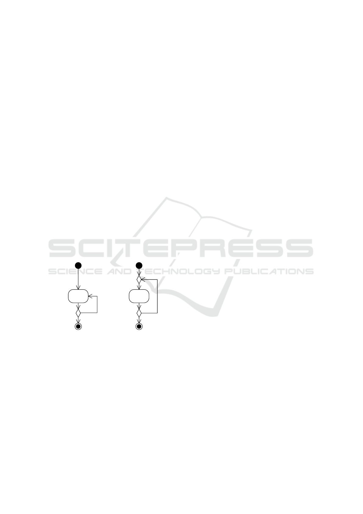
Do
Do
While
MergeNode
While
[true]
[false]
[true]
[false]
Figure 1: Two realizations of a do-while loop as an activity
diagram. Left: UML 1.x, Right: UML 2.x.
Figure 1 shows how a do-while loop would have
been realized in the old and new syntax. If the
UML 1.x version would be run by an fUML execution
engine, the execution would hang with a deadlock af-
ter sending the first token to the Do action, because it
would wait for a second token coming from the deci-
sion node before being able to execute.
Moreover, the fUML specification, being pro-
vided as a Java-like implementation, does not pro-
vide a good mathematical basis for analysis tech-
niques (Laurent et al., 2014).
For these reasons, a verification tool for fUML
models and the execution engine is needed. With
fUML and UML’s activity diagrams based on Petri
net’s token paradigm, and aiming to take advantage of
the already existing literature and methods about Petri
nets verification (Murata, 1989), we decided to bring
the fUML diagrams back to the origin by transform-
ing them to Petri nets. In this way, we can perform
various analyses to check that specific properties hold
within the structure of the model and during its exe-
cution, using the Petri net’s mathematical formalism
as a reliable formal basis.
One result of this paper is a Model-to-model
(M2M) transformation that respects the fUML exe-
cution semantics and provides the foundations for a
lint-like validation tool based on Petri net analysis for
fUML models. This tool will make the modeler aware
of design pitfalls and semantic ambiguities by detect-
ing possible problems that may arise when executing
the diagram sequentially or in parallel.
The following section shows the methodology,
sets the analysis’ goals and briefly surveys different
Petri net analysis techniques. Some related work is
covered along the way. Section 3 shows the trans-
formation rules specific to fUML and how the trans-
formation has been realized. Section 4 gives an ap-
plication example, while results and future work are
discussed in the conclusion section. Finally, the Ap-
pendix covers the proposed set of single transforma-
tion rules.
2 METHODOLOGY
This section at first introduces the issues that we
aim to detect in activity diagrams, followed by an
overview of the primary analysis techniques in Petri
nets that may be used for computing them. We in-
troduce a model-to-model transformation afterwards
and cover some assumptions about the original activ-
ity diagram to allow such a transformation.
2.1 Analysis Goals
Similar to the concept of soundness in the area busi-
ness process modeling (van der Aalst et al., 2000), we
want to make sure that the modeled activity diagrams
have a safe and predictable flow.
For achieving this goal, we would like to analyze
activity diagrams to prove or confute some of the fol-
lowing conditions:
Deadlock is said to happen if the model reaches a
configuration (state) in which no action can fire
(i.e., execute).
Liveness means that the system will keep running,
requiring at least the absence of deadlocks, or the
Towards Automated fUML Model Verification with Petri Nets
299

absence of starvation in some stricter definitions.
Both full and partial liveness covering the whole
or only parts of a model may be of interest.
Unreachable Regions — a set of elements that will
not get executed under certain circumstances, for
example, because they are located after a never-
ending loop.
Problems with concurrent programs falling into
these areas are often rooted in synchronization prob-
lems and caused by erroneous modeling. The ad-
vantage of looking for issues on a Petri net rather
than on the activity diagram directly is that the men-
tioned properties are well researched for Petri net
models, and efficient algorithms for their computation
exist (Sifakis, 1978; Girault and Valk, 2003). More-
over, Petri nets have been introduced for the descrip-
tion of concurrent systems with synchronization, and
should thus be capable of capturing control flow in-
formation of activity diagrams in a natural way.
2.2 Petri Net Analysis
This section will describe possible ways of mapping
the issues listed in Section 2.1 to Petri net properties
and detecting them with algorithm types known for
Petri nets.
The mentioned properties of an activity diagram
can be mapped to similar Petri net properties, pro-
vided that the behavior of the transformed model is
identical:
Deadlocks a deadlock occurs in a Petri net when no
transition can fire due to the lack of (one or more)
input tokens.
Liveliness Petri net transitions and nets have sev-
eral levels of liveliness (L
0
: dead - L
4
: live) (Gi-
rault and Valk, 2003) that can be mathematically
proved.
Unreachable Regions a set of transitions that will
not fire because of missing tokens in a state reach-
able by the initial net marking.
Moreover, it is possible to analyze the net’s bound-
edness to check if the amount of tokens in the net re-
mains bounded, which may otherwise point at infinite
loops or wrong recursion steps.
Provided that a behavioral similar model has been
created, the next step is to compute the properties
with existing analysis methods. Reachability anal-
ysis, which consists of enumerating and analyzing
all reachable states of a net, does not scale for big-
ger models or unbounded networks with an unlimited
number of states. This issue is known as the state
space explosion problem (Valmari, 1998).
A linear algebraic analysis approach would lead to
a similar problem, resulting in many linear equations
to consider.
It would be then possible to apply some trans-
formation techniques to simplify the Petri net mak-
ing the analysis process more straightforward, but
then the difficulty would be finding the reducible sub-
networks and then backtracking the error to the origi-
nal element.
Synthesis methods for reducing the size of Petri
nets are NP-complete (Badouel et al., 2015) and can-
not cope with strongly coupled subsystems.
Simulating the Petri net often requires long run
times, and does not assure that all possible markings
are covered. This well-known principal problem of
simulation algorithms is similar to the test coverage
problem.
Graph theoretical analysis (for example, looking
for siphons and traps (Murata, 1989)) are inexpensive
but may detect false-positives too. For instance, activ-
ity initial and final nodes would be detected as siphons
and traps, respectively.
For these reasons the authors argue that a graph
theoretical analysis should be preferred over the other
methods, as it is less expensive to compute and pro-
vides satisfying hints about possible problems in the
net. Those hints can then be analyzed individually
with a heuristic to filter out possible false positives.
2.3 Activity Diagram Transformation to
Petri Nets
With the UML activity diagram specification based
on Petri nets semantics (OMG, 2017b), the trans-
formation of activity diagrams elements to Petri net
snippets should be quite natural from a conceptual
point of view. Similar transformation approaches
have been reported in the literature, although with dif-
ferent goals.
The transformation can be performed to evaluate
program performance as in (Distefano et al., 2011)
and (López-Grao et al., 2004), where UML 1.x activ-
ity diagrams are transformed to stochastic Petri nets to
evaluate their performance. This technique can also
be applied to compute other properties of the mod-
eled system. For example, system execution time and
number of resources that the system would consume
are simulated in (Andrade et al., 2009). This approach
is based on SysML activity diagrams transformed into
Time Petri nets to validate the requirements of embed-
ded systems.
Our goal and approach are more similar to the
one introduced in (Agarwal, 2013), which proposed
a method for transforming the essential elements of
MODELSWARD 2019 - 7th International Conference on Model-Driven Engineering and Software Development
300

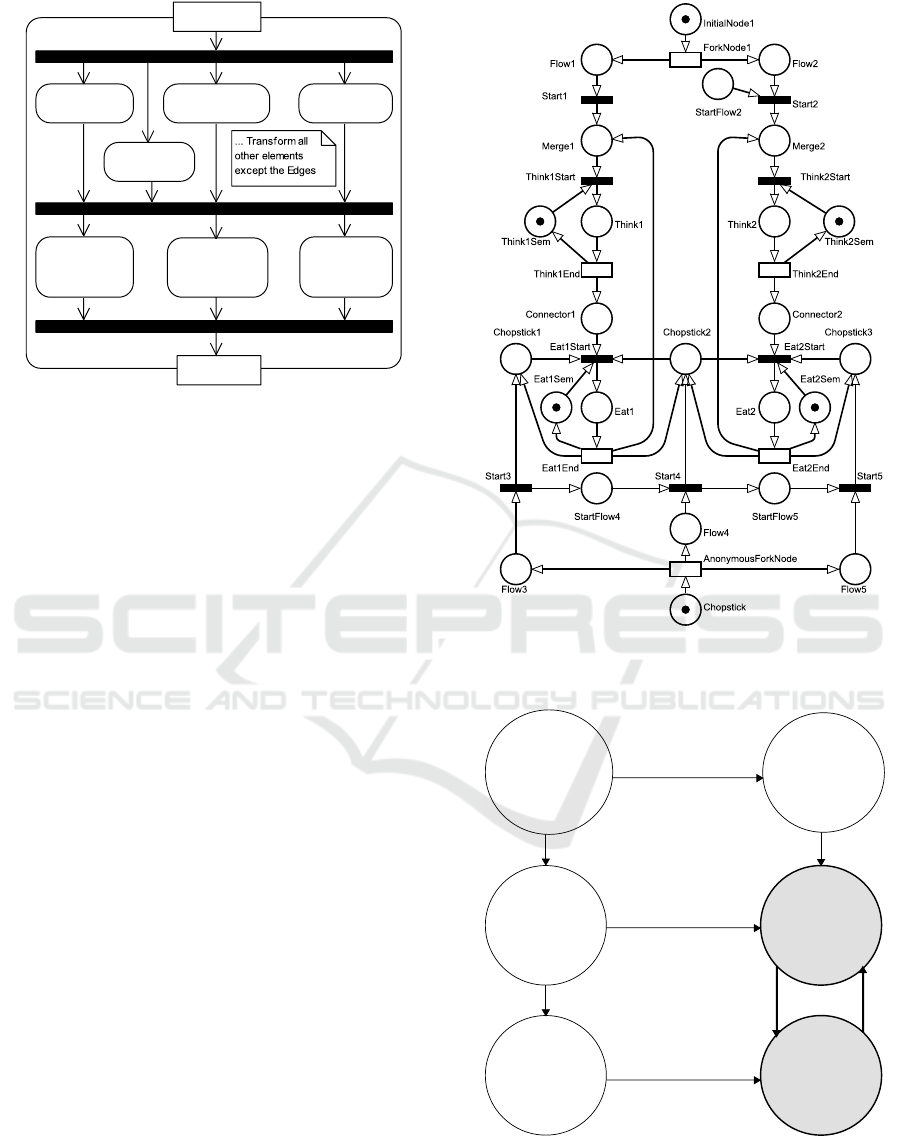
HaveDinner
Think
Eat
Think
Eat
<<centralBuffer>>
Chopstick2
<<centralBuffer>>
Chopstick1
<<centralBuffer>>
Chopstick3
Chopstick
InitialNode
ForkNode
Merge1
Merge2
Figure 2: An activity diagram modeling the dining philoso-
pher problem with only two philosophers.
UML 2.x activity diagrams. The goal there is to
analyze the diagrams’ liveliness, boundedness, and
reachability for verification purposes. The transfor-
mation methods we used are also similar to the in-
tuitive ones covered in (Staines, 2008) and (Störrle,
2004). The transformation rules we used are dis-
played in the appendix for completeness.
2.3.1 fUML Specification Issues
To demonstrate the issues which arise by applying the
existing transformations to fUML activity diagrams,
let us consider the well-known Dining Philosopher
problem (Andrews, 1991) as a kind of benchmark for
concurrent system design. Figure 2 shows, for sim-
plicity, a section with just two philosophers (as mod-
els for concurrent processes) who are having dinner.
For simplicity, we allow in the model the philoso-
phers to take both chopsticks with one atomic action,
such that at least deadlocks cannot happen according
to the requirements of deadlocks in concurrent sys-
tems. The execution starts and two identical flows
start to run. Each philosopher is thinking at the be-
ginning. Then, if both chopsticks are available, they
can eat (one at a time) and go back to thinking after-
wards.
The changes introduced by the fUML specifica-
tion regarding the fixed order of execution of the
model profoundly changed the semantics depicted
initially by UML 2.x, in a way that can be mislead-
ing for some modelers.
Due to the depth-first approach and the strict
ordering intrinsically modeled in the fUML spec-
ification (inside the function ActivityNode-
Activation::sendOffers), the first merge node
that gets executed keeps running forever, leading the
other philosopher to starvation. Which one is the first
depends on the order how the fork node edges have
Figure 3: A Petri net representing the activity diagram in
Figure 2, obtained using the intuitive transformation.
been saved or on the order how the execution engine
internally stores them, which is a low-level technical
issue that should not influence the model behavior.
With just two philosophers, it would be possible
to solve this problem by using a decision node that
randomly picks one of its two outgoing edges instead
of the fork node. Unfortunately, this solution would
not scale with more philosophers (only one would be
allowed to eat at any time), and it requires the modeler
to include a scheduling detail in its model instead of
focusing on the high-level concurrent design of the
problem.
UML 2.x specified that concurrent execution
means that there is no required order in which the
nodes must be executed; a conforming execution of
the Activity may execute the nodes sequentially in ei-
ther order or may execute them in parallel (OMG,
2017b). fUML adheres to this specification by execut-
ing one of them first but never gets to execute the sec-
ond one until the first one finishes (and that is never
going to happen in our example).
If we would transform the activity diagram in
Figure 2 to a Petri net following the intuitive trans-
formation based on the UML 2.x specification, we
would obtain the diagram shown in Figure 3, which
would be correct concerning the original semantics of
UML 2.x, but not according to the new sequentialized
execution semantics of fUML.
Analyzing this Petri Net would not lead to dis-
covering any problem. The model executes as ex-
pected, both processes execute concurrently, and both
Towards Automated fUML Model Verification with Petri Nets
301
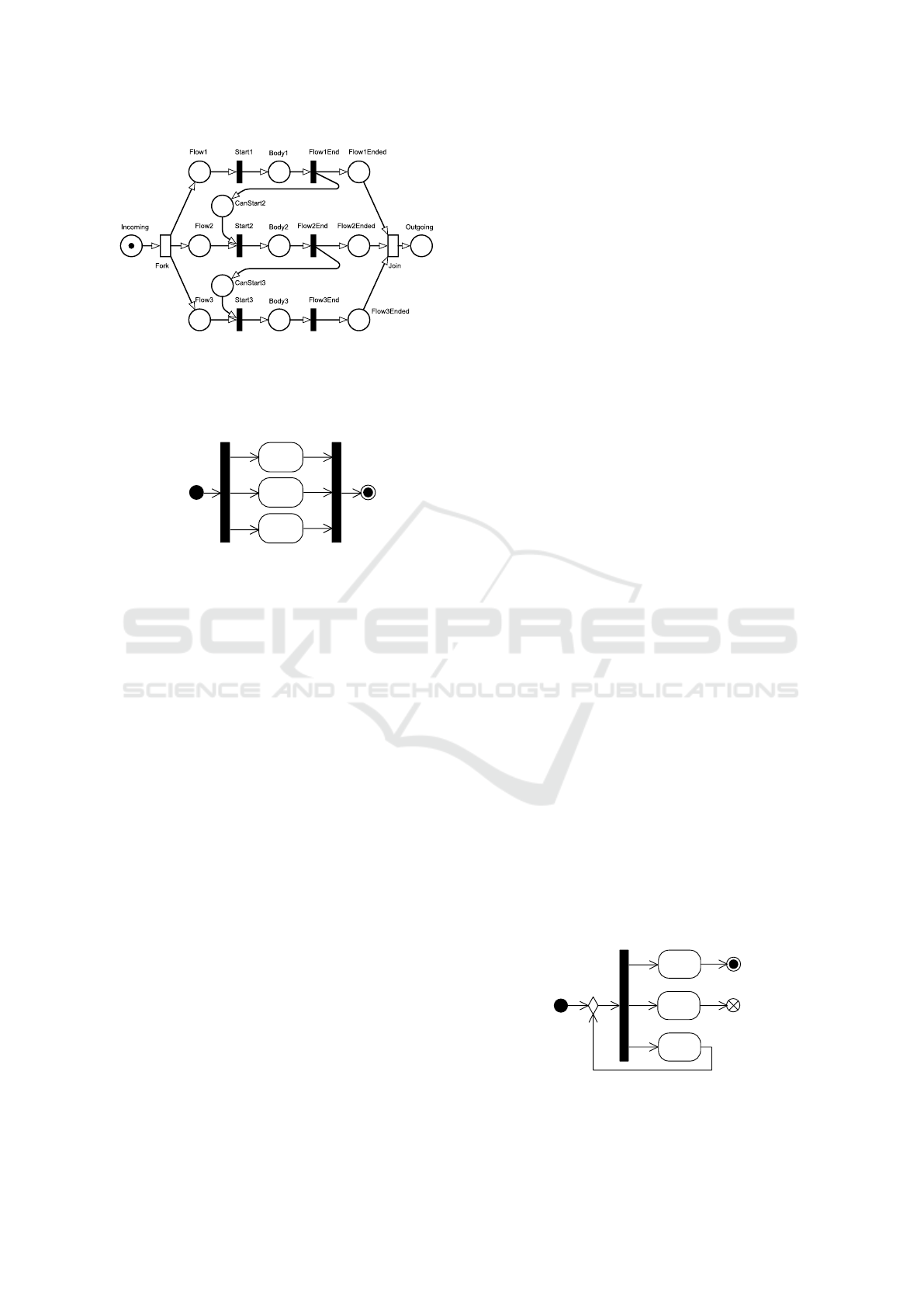
Figure 4: A Petri net realizing fUML a fork and join con-
struct with a sequential execution. The three body places
are just placeholders; in reality, actions are not transformed
as a single place, but as a set of elements (as presented in
the Appendix).
Body1
Body2
Body3
Figure 5: An activity diagram showing a fork and join of
three flows.
philosophers will eventually be eating. However, it
does not resemble the specified fUML behavior and
thus does not show problems arising from it. For this
reason, we introduce a different kind of transforma-
tion, to resemble fUML’s strict sequential execution
of fork node flows.
2.3.2 Sequential Transformation of Fork Nodes
This section proposes an fUML-conform transforma-
tion technique for transforming fork nodes to Petri
nets. The proposed transformation replicates the
fUML sequential execution of fork nodes outgoing
flows, to be able to detect problems that would happen
during the sequential execution of activity diagrams.
Figure 4 shows our proposed transformation for
the activity diagrams in Figure 5.
We introduce two additional immediate transitions
for each flow that should fire at the beginning and the
end of the flow. For this to happen, we need one addi-
tional place (CanStart#) for all flows (except the first
one), that shall receive one token once the previous
flow finishes its execution. The FlowEnd transition
takes care of placing this token.
In case a flow does not end (for example when
it contains an infinite loop), the CanStart place of
the following flow will not receive a token, clearly
marking the remaining flows as unreachable inside
the Petri net. Moreover, looking for the end (or ends)
of the flows allows us to locate critical sections or
loops in the model already during the transformation
phase.
It is evident that the Flow2 and Flow3 places and
the Fork transition itself are redundant and could be
left out in this diagram without missing anything in
the final analysis. However, to make the recognition
of the different flows simpler and their structure more
systematic, we have decided to still include them in
the transformation. Additionally, when those places
are identified as traps, we can warn the user more pre-
cisely about which flow will encounter problems.
Finding the final element of a flow is not trivial
and will be solved in future work. At this time, we can
simplify this task by saying that a join or flow final or
activity final nodes would resemble, for example, an
obvious end of the flow.
Another problem that arises is that the order used
during the execution is implementation-specific and
depends on different factors, such as how the elements
get saved inside the fUML model, and how the exe-
cution engine reads and stores the edges (in a FIFO or
a LIFO data structure, for example).
For example, in Figure 6 a peculiar but syntacti-
cally valid fork node with three actions is shown. De-
pending on which flow gets executed first, it is possi-
ble to obtain several different results:
A executes first: the action A executes once, and the
activity ends, reaching the activity final node.
B executes first: the action B executes once and
then, depending on the internal ordering, either A
gets executed once, or C gets executed in an infi-
nite loop with B (B, C, B, C. . . ).
C executes first: results in an infinite loop of C ac-
tions (C, C, . . . ).
These examples show that although the fUML
goal was to be specific enough to provide a
precise semantic for consistent execution flows,
implementation-specific details can still produce dif-
ferent results while running the same model. To use
the proposed sequentialized transformation, the M2M
transformation either requires some extra knowledge
A
B
C
Figure 6: An activity diagram showing one fork node with
three outgoing flows. Its execution heavily depends on the
specific execution engine implementation.
MODELSWARD 2019 - 7th International Conference on Model-Driven Engineering and Software Development
302

about the implementation-specific peculiarities of the
fUML execution engine or should produce all possi-
ble combinations and analyze all of them.
2.4 Transformation Assumptions
For the analysis, we require the following assump-
tions or limitations for activity diagrams to allow
them to be transformable:
Assumption 1. All actions must terminate and pro-
duce the outputs they are expected to provide on their
output edges, even if empty.
This restriction is necessary because the transfor-
mation loses some information about the behavioral
semantics of the original model, which is possible to
model in different ways (for example as programming
code inside a function behavior), and it is not possible
to easily transfer it into a Petri net. For this reason,
our analysis must assume that actions never hang and
always produce a token on all their outgoing edges.
Informally, the transformation cannot take a look “in-
side” the actions, and thus the significant behavior
must be clear from the model structure.
Assumption 2. Actions should not modify at-
tributes that may get used by other actions which may
run concurrently during their execution.
For the same reasons of Assumption 1, all actions
must resemble an atomic set of operations. Activity
diagrams are high-level descriptions of a process, and
only elements that are explicitly present in a model
can be analyzed. Therefore it is important to not
hide too much logic behind actions, which can be ex-
pressed using other activity diagrams elements.
Assumption 3. Activity diagrams may consist of a
set of supported elements only. This set consists of ac-
tivity initial and final nodes, activity input and output
parameters, flow final nodes, decision nodes, merge
nodes, fork and join nodes, central buffer nodes, data-
store nodes, actions with input and output pins and
loop nodes.
If the diagrams contain unsupported parts such as
event-related elements (i.e., send/receive signal ac-
tions and time events), they will not be transformed,
and the analysis would take place on an incomplete
diagram probably leading to wrong or at least only
partial results.
Assumption 4. The input model is syntactically
valid, which implies that all elements are correctly
connected with control or object flows. As the trans-
formation considers both data and control flows as
one single kind of tokens, it is essential that the origi-
nal model allows to transfer them correctly.
3 REALIZATION
To implement the transformation, we have used op-
erational QVT (QVTo), whereas for performing the
Petri net analysis, we are using the existing tool
TimeNET (Zimmermann, 2017). QVTo is an OMG
standard using an OCL-like imperative language, be-
ing still actively developed and well integrated into
Eclipse (Tikhonova and Willemse, 2015). It works
following the Query/View/Transformation paradigm,
requiring to first selecting (query) from the original
model the elements which will be transformed, then
define how they should look like (view) in the output
model by defining a transformation that realizes it.
The exogenous model-to-model transformation
from activity diagrams to Petri nets requires the
source and the destination meta-models. For UML we
used the UML ecore meta-model available from the
core Eclipse Modeling Framework (EMF), whereas
for the Petri net meta-model we have generated the
ecore meta-model from TimeNET’s internal XML
schema files (XSD) specifying stochastic Petri nets.
In TimeNET, this schema does not only describe
Extended Deterministic and Stochastic Petri nets, but
represents a model class containing the modeling
power of several well-known sub-classes like GSPNs,
DSPNs, and eDSPNs (Zimmermann, 2007) allowing
different transition firing delay types. This extended
set allows us not to be restricted a priori to a single
class of Petri nets, leaving us the possibility to extend
or switch to a different subclass of Petri net when new
analysis methods are needed.
Once the input and output meta-models are avail-
able, the input model can be provided to a transforma-
tion tool, which will execute an ordered set of trans-
formation rules (also known as mappings) to produce
a Petri net model.
QVTo uses a hierarchical waterfall approach,
where a linear sequence of steps obtains the trans-
formed model. The transformation operates as illus-
trated in Figure 7. However, due to QVTo’s limita-
tions, the transformation is implemented sequentially
and operates as follows:
1. Transform firstly all the single activity diagram’s
nodes (for the transformation details, refer to the
Appendix).
2. Transform all edges between elements:
Towards Automated fUML Model Verification with Petri Nets
303
Transform AD2PNm
Transform Initial
Nodes
Transform Activity
Parameter Nodes
Transform Fork
Nodes
Transform Flow
Final Nodes
Transform Edges
with additional
Places
Transform Edges
with additional
Transitions
Transform
remaining Edges
fUML Model
Petri Net Model
Figure 7: Activity diagram showing the required steps for
transforming an fUML activity diagram to a Petri net with
QVTo.
(a) transform all edges which require an extra tran-
sition (between two places);
(b) transform all edges which require an extra place
(between two transitions);
(c) transform the remaining edges (between a place
and a transition, and vice versa).
With the transformation process in place, the ac-
tivity diagrams can be now translated to Petri nets.
This transformation is not complete and loses a part
of the original model semantics, for instance the ac-
tions’ function behaviors which are internally defined
as source code. On the other hand, the transformation
allows us to perform more advanced analysis on the
general structure of the diagram.
4 EXAMPLE
This section describes how the proposed sequential
Petri net transformation can detect starvation in the
philosophers problem previously described in Sec-
tion 2.3.
It is possible to apply different techniques to ana-
lyze the resulting Petri net shown in Figure 8. For ex-
ample, a structural analysis of the net shows that the
sets of places {Merge1, Think1, Connector1, Eat1}
and {Merge2, Think2, Connector2, Eat2} are traps,
denoting the presence of possible never-ending loops.
Petri net traps are sets of places which may receive
additional tokens, but will never allow them to leave
the trap.
Using the TimeNET tool, the reachability graph
(Figure 9) can be computed. It shows that there is an
Figure 8: A Petri net showing the result of the proposed se-
quentialized transformation of the fUML model in Figure 2
InitialNode, Chopstick,
Eat1Sem, Eat2Sem,
Think1Sem, Think2Sem
Flow2, Chopstick,
Eat1Sem, Eat2Sem,
Think1, Think2Sem
InitialNode,
Chopstick1,
Chopstick2,
Chopstick3, Eat1Sem,
Eat2Sem,
Think1Sem,
Think2Sem
Connector1,
Chopstick, Eat1Sem,
Eat2Sem, Flow2,
Think1Sem,
Think2Sem
Chopstick3, Flow2,
Eat1, Eat2Sem,
Think1Sem,
Think2Sem
Flow2, Chopstick1,
Chopstick2,
Chopstick3, Eat1Sem,
Eat2Sem,
Think2Sem, Think1
Think1End,
Eat1Start
Eat1End,
Think1Start
AnonymousForkNode, Start3,
Start4, Start5, Eat1Start
Think1End
AnonymousForkNode,
Start 3, Start4, Start5
ForkNode, Start1,
Think1Start
AnonymousForkNode,
Start 3, Start4, Start5
ForkNode, Start1,
Think1Start
Figure 9: The reachability graph of the Petri net shown in
Figure 8. Inside the circles, places who hold exactly one
token are listed, while transitions causing state changes are
shown on the arcs. The grey elements visualize a loop.
MODELSWARD 2019 - 7th International Conference on Model-Driven Engineering and Software Development
304

infinite loop between two states, which hints to the
same (potential undesired) condition in the original
diagram. Moreover, as some transitions are never fir-
ing in the reachability graph, some parts of the model
containing the missing transitions are unreachable
from the initial marking (Think2Start and Eat2Start
in the example).
The shown steps demonstrate that difficulties in
transforming an activity diagram into a Petri net arise
from the incomplete specification of such diagrams,
but that execution-specific issues can be detected with
a correctly extended Petri net that incorporates the se-
quential fUML execution.
5 CONCLUSION
In this paper, we have developed the foundation for
a lint-like fUML activity diagram verification, which
can be used to detect and warn modelers about er-
rors or potentially dangerous anomalies in their di-
agrams describing concurrent programs. This ap-
proach is based on two types of M2M transformations
to Petri nets: 1) an intuitive one similar to the exist-
ing literature to tackle conceptual problems, and 2) an
fUML-conform one introduced here to find problems
caused by the sequential execution semantics speci-
fied by the fUML. In particular, our method with its
different transformations, aims to detect synchroniza-
tion problems that would occur when the diagrams are
executed both concurrently and sequentially.
The sequential transformation of fork nodes al-
lowed us to verify not only models that were ob-
viously wrong (for example with disconnected ele-
ments), but also models without such problems that
in reality lead to a peculiar execution which is hard
to predict without expert knowledge of the execution
engine implementation.
As a side effect, the paper points out current limi-
tations and potentially dangerous situations of the cur-
rent fUML specification, that would only become evi-
dent when the execution happens concurrently or with
a different static execution order.
5.1 Future Work
The next steps consist of finding a suitable algorithm
for correctly transforming all possible constellations
of fork node flows; i.e., finding or deciding the ab-
sence of the end of each flow. Once a reliable method
is defined, it will be possible to implement the sequen-
tial transformation of fork node flows.
Further work will include parallelization of the
fUML C++ execution engine developed in our group
(MDE4CPP, (Bedini et al., 2017)), automation of the
M2M transformation, and the execution of the analy-
sis techniques which are relevant to the input model.
The transformation implementation is available
online
1
and distributed under the MIT license.
REFERENCES
Agarwal, B. (2013). Transformation of UML Activity Dia-
grams into Petri Nets for Verification Purposes. Inter-
national Journal Of Engineering And Computer Sci-
ence, 2(3):798–805.
Andrade, E., Maciel, P., Callou, G., and Nogueira, B.
(2009). A methodology for mapping sysml activity
diagram to time petri net for requirement validation of
embedded real-time systems with energy constraints.
In 2009 Third International Conference on Digital So-
ciety (ICDS), pages 266–271.
Andrews, G. R. (1991). Concurrent programming: prin-
ciples and practice. Benjamin/Cummings Publishing
Company San Francisco.
Arlow, J. and Neustadt, I. (2002). UML 2 and the Unified
Process: Practical Object-Oriented Analysis and De-
sign. Pearson Education, Inc., 2 edition.
Badouel, E., Bernardinello, L., and Darondeau, P. (2015).
Petri net synthesis. Springer.
Bedini, F., Maschotta, R., Wichmann, A., Jäger, S., and
Zimmermann, A. (2017). A model-driven fuml exe-
cution engine for C++. In Proceedings of the 5th In-
ternational Conference on Model-Driven Engineering
and Software Development, MODELSWARD 2017,
Porto, Portugal, February 19-21, 2017., pages 443–
450. SciTePress.
Distefano, S., Scarpa, M., and Puliafito, A. (2011). From
UML to Petri Nets: The PCM-Based Methodol-
ogy. IEEE Transactions on Software Engineering,
37(1):65–79.
Eshuis, R. and Wieringa, R. (2004). Tool support for ver-
ifying uml activity diagrams. IEEE Transactions on
Software Engineering, 30(7):437–447.
Girault, C. and Valk, R. (2003). Petri Nets for System Engi-
neering. Springer.
Laurent, Y., Bendraou, R., Baarir, S., and Gervais, M.-P.
(2014). Formalization of fuml: An application to pro-
cess verification. In International Conference on Ad-
vanced Information Systems Engineering, pages 347–
363. Springer.
López-Grao, J. P., Merseguer, J., and Campos, J. (2004).
From UML Activity Diagrams to Stochastic Petri
nets: application to software performance engineer-
ing. ACM SIGSOFT Software Engineering Notes,
29(1):25–36.
Murata, T. (1989). Petri nets: Properties, analysis and ap-
plications. Proceedings of the IEEE, 77(4):541–580.
OMG (2017a). fUML 1.3 Specifications.
https://www.omg.org/spec/FUML/1.3/PDF. on-
line.
1
https://github.com/MDE4CPP/AD2PN
Towards Automated fUML Model Verification with Petri Nets
305
OMG (2017b). Unified Modeling Lan-
guage, Specification version 2.5.1.
https://www.omg.org/spec/UML/2.5.1/PDF. on-
line.
Sifakis, J. (1978). Structural properties of Petri nets. In
Winkowski, J., editor, Mathematical Foundations of
Computer Science, pages 474–483. Springer Verlag.
Staines, T. S. (2008). Intuitive Mapping of UML 2 Activity
Diagrams into Fundamental Modeling Concept Petri
Net Diagrams and Colored Petri Nets. In 2008 15th
Annual IEEE International Conference on Engineer-
ing of Computer Based Systems (ECBS), pages 191–
200.
Störrle, H. (2004). Semantics of control-flow in uml 2.0
activities. In 2004 IEEE Symposium on Visual Lan-
guages - Human Centric Computing, pages 235–242.
Störrle, H. (2005). Semantics and verification of data flow
in uml 2.0 activities. Electronic Notes in Theoretical
Computer Science, 127(4):35 – 52. Proceedings of the
Workshop on Visual Languages and Formal Methods
(VLFM 2004).
Störrle, H. and Hausmann, J. H. (2005). Towards a formal
semantics of uml 2.0 activities. In Software Engineer-
ing.
Tikhonova, U. and Willemse, T. (2015). Designing and de-
scribing qvto model transformations. In 2015 10th
International Joint Conference on Software Technolo-
gies (ICSOFT), volume 1, pages 1–6.
Valmari, A. (1998). The state explosion problem, pages
429–528. Springer Berlin Heidelberg, Berlin, Heidel-
berg.
van der Aalst, W., Desel, J., and Oberweis, A. (2000). Busi-
ness Process Management — Models, Techniques, and
Empirical Studies. LNCS 1806. Springer Berlin Hei-
delberg.
Zimmermann, A. (2007). Stochastic Discrete Event Sys-
tems — Modeling, Evaluation, Applications. Springer,
Berlin Heidelberg New York.
Zimmermann, A. (2017). Modelling and performance eval-
uation with TimeNET 4.4. In Bertrand, N. and Borto-
lussi, L., editors, Quantitative Evaluation of Systems
- 14th Int. Conf., QEST 2017, pages 300–303, Berlin,
Germany.
APPENDIX
fUML Activity Diagram to Petri Net
Transformation
This appendix shows how the QVTo transformation
translates the single fUML elements to Petri nets us-
ing the intuitive transformation.
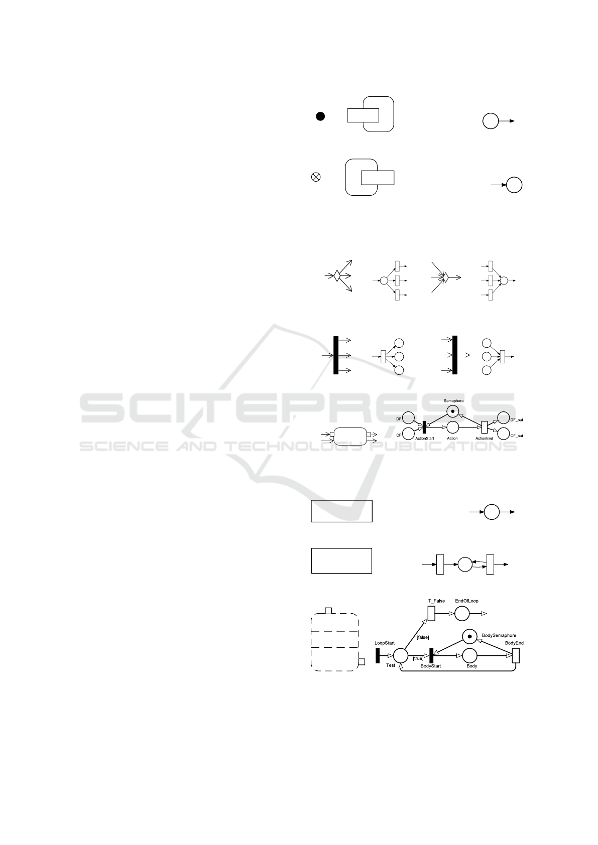
Activity
Input
or
●
Activity Initial Node / Activity input parameter.
Activity
Output
or
Flow Final node / Activity Output Parameter. An Activity
Final node may be translated in the same way, but it would
not have the same semantic meaning as in an activity dia-
gram.
Decision/Merge nodes with 3 flows.
Fork/Join nodes with 3 flows (intuitive transformation).
Action
A Call Behavior/Operation Action, with incoming and out-
going data and control flows. The semaphore allows to ex-
ecute the action multiple times in a loop with the correct
number of input parameters.
<<centralBuffer>>
CentralBufferNode
A Central buffer node.
<<datastore>>
DataStoreNode
DF
A Data Store Node with one input and one output flow.
<<structured>>
Loop
Test
Body
A Loop Node. According to the fUML specification, its
Setup section must be empty.
MODELSWARD 2019 - 7th International Conference on Model-Driven Engineering and Software Development
306
