
A Cellular Automata based Classification Algorithm
Tu
˘
gba Usta
1
, Enes Burak D
¨
undar
2
and Emin Erkan Korkmaz
1
1
Department of Computer Engineering, Yeditepe University,
˙
Istanbul, Turkey
2
Department of Computer Engineering, Bo
˘
gazic¸i University,
˙
Istanbul, Turkey
Keywords:
Classification, Cellular Automata, Big Data.
Abstract:
Data classification is a well studied problem where the aim is to identify the categories in the data based on a
training set. Various machine learning methods have been utilized for the problem. On the other side, cellular
automata have drawn the attention of researchers as the system provides a dynamic and a discrete model for
computation. In this study a novel approach is proposed for the classification problem. The method is based
on formation of classes in a cellular automata by the interaction of neighborhood cells. Initially, the training
data instances are assigned to the cells of a cellular automaton. The state of a cell denotes the class assignment
of that point in the instance space. At the beginning of the process, only the cells that have a data instance
have class assignments. However, these class assignments are spread to the neighbor cells based on a rule
inspired by the heat transfer process in nature. The experiments carried out denote that the model can identify
the categories in the data and promising results have been obtained.
1 INTRODUCTION
Given a set of training examples
{(x
1
,l
1
),(x
2
,l
2
),...(x
n
,l
n
)}, where x
i
is a data
instance represented as a feature vector and l
i
is the
corresponding class label for x
i
, the classification
task can be defined as inducing a function f : X → L
where X is the instance space and L is the output
space. The accuracy of the process is determined
by using a separate test set. The f function can be
considered as a separator in the instance space that
can distinguish the categories in the data. Various
techniques have been proposed and utilized for
classification problems including decision trees,
support vector machines or Bayesian approaches
(Friedl and Brodley, 1997; Cortes and Vapnik,
1995; Cheeseman et al., 1988). Cellular Automata
(CA) provides a means for computation based on a
discrete system that is composed of interconnected
cells. The Conway’s Game of life is the most well
known example for CA (Gardner, 1970). Other CA
applications exist in the literature where CA have
been mainly used as simulation tools for various
disciplines (Ermentrout and Edelstein-Keshet, 1993;
Hesselbarth and G
¨
obel, 1991; Mai and Von Niessen,
1992; Margolus et al., 1986; Langton, 1984)
Classification techniques that utilize different
types of CA have also been proposed in the literature.
For instance in (Povalej et al., 2005), a Multiple Clas-
sifier System is proposed. In the study, an automaton
is used to determine the set of appropriate classifiers
for a specific problem. In (Esmaeilpour et al., 2012),
a learning CA is proposed to extract the patterns in the
raw data. The learning process that takes place in the
automaton detects the frequently repeated patterns in
the data.
The two studies mentioned above utilize CA in
the classification process for different purposes. How-
ever, in (Kokol et al., 2004), the classification process
is carried out by a CA. An energy function is utilized
and the features of the dataset are associated with the
columns of the CA. The energy value of a cell in a cer-
tain column denotes if a training sample is classified
correctly or not. The learning is carried out by the in-
teraction of the neighbor cells. The energy parameter
and threshold values utilized in the study needs to be
tuned for each dataset separately and this is a serious
drawback for the study.
In this study, a stochastic cellular automata algo-
rithm named as SCA-classification is proposed and
the method classifies the data again by using a CA. At
the beginning of the procedure, the elements in the
training dataset are mapped to fixed cells in a CA.
Then each cell is assigned a state number denoting
the class label of the data instance it contains. Cer-
tainly, the empty cells will have no class assignments,
initially. Then, by using the local interactions among
the cells, the class labels are transferred to the other
cells in the automaton. The process of spreading the
class labels is inspired by the heat transfer process in
nature. The CA cells that have a data instance are con-
Usta, T., Dündar, E. and Korkmaz, E.
A Cellular Automata based Classification Algorithm.
DOI: 10.5220/0007373001550162
In Proceedings of the 8th International Conference on Pattern Recognition Applications and Methods (ICPRAM 2019), pages 155-162
ISBN: 978-989-758-351-3
Copyright
c
2019 by SCITEPRESS – Science and Technology Publications, Lda. All rights reserved
155

sidered as heat sources and they generate heat energy
continuously. This energy is spread to the neighbor-
hood cells and the regions that are close to the data in-
stances warm up in the automaton. On the other side,
a second rule is used which enables the heated cells
to change their states. Hence, the cells without class
assignments start to join different classes represented
by different states in the automaton. In the end, the
instance space represented by the automaton is cate-
gorized based on the classes that exist in the training
data.
The idea of using heat propagation in a CA to
perform certain kind of computations has been ap-
plied to the clustering problem in (D
¨
undar and Kork-
maz, 2018). Clustering is a also well studied problem
where the process is carried out on unlabelled data, in
an unsupervised manner. Even though a similar heat
propagation approach is utilized in (D
¨
undar and Ko-
rkmaz, 2018), the data is analyzed with a different al-
gorithm in order to determine the clusters in the data.
Hence, the two studies differ from each other espe-
cially in terms of the state transfer rule and the termi-
nation criteria utilized. The approach used in (D
¨
undar
and Korkmaz, 2018) forms different primitive clusters
in the CA and then these primitive units are combined
into larger clusters in order to obtain the final clus-
tering of the dataset. In (Uzun et al., 2018), a similar
approach has been proposed to solve the classification
problem. However, this study utilizes a separate two
dimensional CA for each class and each feature in the
dataset is separately analyzed by the method.
The approach proposed in this study has also simi-
larities with the method presented in (Fawcett, 2008).
The authors utilize CA for the classification process in
(Fawcett, 2008), too. However, they use a voting rule
where a cell changes its state according to the major-
ity class among its neighbors. In (Fawcett, 2008), it is
noted that each cell is assigned to the class label of the
nearest initial point in the CA according to Manhattan
Distance. In our study, a different framework is uti-
lized for changing the cell states. As noted above, the
process is inspired from the heat transfer procedure in
nature. This provides a different inductive bias where
the structure of classes formed is dependent on the
distribution of the data in the CA. Details about the
differences between the two approaches can be found
in section 3.
2 METHODOLOGY
Cellular Automata provide a dynamical system which
is composed of regular cells. Each cell in the system
can be in one of a predefined set of states and com-
putation is carried out by updating the state values by
some specific rules. These rules are defined based on
the interaction of neighbor cells.
(a) Moore (b) Von Neumann
Figure 1: Neighborhood Types.
The two most commonly used neighborhood types
in the model are the Moore neighborhood and Von
Neumann neighborhood. In 2-dimensions, the cen-
ter cell has 8 neighbors according to Moore neighbor-
hood. As seen in Figure 1a, if the center cell is C
i, j
,
then all cells C
k,s
where |i −k| ≤ 1 or | j −s| ≤ 1 would
be in the Moore neigborhood of the center cell. In a n
dimensionsional CA, the center cell would have 3
n
−1
neighbors. On the other side, the center cell has only 4
neighbors in 2 dimensions according to Von Neumann
neighborhood. As seen in Figure 1b, if the center cell
is C
i, j
, then only the cells C
k,s
where |i − k| = 1 and
| j − s| = 0 or |i − k| = 0 and | j − s| = 1 would be in
the neigborhood. This time, in n dimensions, the cen-
ter cell has 2 ∗ n neighbors. In Moore neighborhood,
the number of neighbor cells increase exponentially
based on the dimension, however this increase is lin-
ear in Von Neumann neighborhood. Therefore, Von
Neumann neighborhood is used in this study.
2.1 Assigning Data Instances to CA
Cells
The instances in the dataset have to be assigned to the
cells of a CA at the beginning of the procedure. The
CA utilized for the process would have n dimensions
where n is determined by number of attributes in the
dataset. The dataset is separated randomly into train-
ing (60%), test (20%) and validation (20%) sets ini-
tially. Certainly, the test set is utilized for determining
the success rate after the training process is finished.
The validation set is utilized for defining a termina-
tion criterion for the training phase (The details can
be found in Section 2.4).
A data instance is assigned to a CA cell based on
its attribute values. If the number of cells in dimen-
sion d is c and if the maximum and minimum values
of the attribute associated for this dimension are A
d
max
and A
d
min
in the dataset, then in this dimension, the
index of the cell (x
i
d
) for a data instance x that has at-
tribute value x
d
A
, is calculated as given in Equation 1.
ICPRAM 2019 - 8th International Conference on Pattern Recognition Applications and Methods
156
In this equation, the ceiling function is needed since
the calculated indexes are integer values.
x
i
d
=
l
x
d
A
− A
d
min
(A
d
max
− A
d
min
)/c
m
(1)
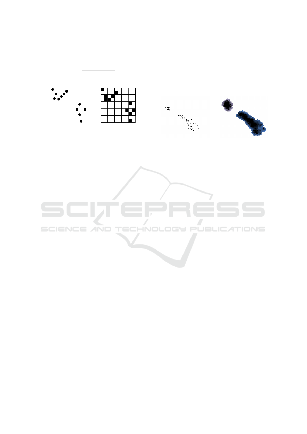
(a) A sample dataset (b) Data instances
assigned to cells
Figure 2: Mapping process for 2-dimensional sample data.
An example mapping process is illustrated in Fig-
ure 2. In Figure 2a, a sample dataset distribution is
presented. Then the data instances are mapped to
the lattice according to attribute values in Figure 2b.
Certainly, the cell indexes are calculated by using the
Equation 1. The empty cells would not have any class
assignment initially. As noted in the previous section,
the class labels are spread in the CA by a method in-
spired from the heat transfer process in nature. The
cells that contain data instances are considered as heat
sources. The heat energy which is generated by these
cells is transferred to other cells. Therefore, each cell
has also an initial temperature value. The cells that
contain data instances have fixed temperature 100
◦
.
The empty cells have 0
◦
temperature at the beginning
of the procedure. Two different rules are utilized in
the classification process. The first rule transfers the
heat energy produced by the heat sources in the au-
tomaton. The second rule enables the warmed empty
cells to change their state. When these two rules are
utilized on randomly chosen cells repeatedly, the class
labels represented by the state values of the initial
cells start to spread to the empty cells in the CA and
it becomes possible to categorize the instance space
represented by the CA. These two rules are presented
in detail in the next two subsections.
2.2 Heat Transfer in CA
The heat transfer rule is given in algorithm 1. The in-
put cell C in the algorithm is selected randomly from
a selection set. The selection set consists of the cells
with data instances and their neighbors initially. Then
the neighbors of the selected cell are determined. If a
neighbor does not exist in the selection list, it is also
created and added to the data structure (which means
it can be also selected for heat transfer procedure in
the following steps). Then the average temperature of
the selected cell and its neighbors is determined. Note
that if the cell contains a data instance, its temperature
is fixed (100
◦
) and it is not updated by the procedure.
However, if the cell is empty, its new temperature is
set as the average value. What is more, the tempera-
ture of the neighborhood cells are also updated unless
they contain a data instance.
(a) Initial data distribution (b) Heat propagation
Figure 3: Heat propagation process.
The average temperature of all cells would have
a tendency to be equalized with the above procedure.
However, the heat sources constantly provide energy
to the system and they do not cool down. This enables
the regions with more data instances to be heated
more compared to other regions in the CA. In Figure
3a, an example 2-dimensional dataset is given. Fig-
ure 3b presents the temperature values of CA cells af-
ter the above procedure is applied for a while on ran-
domly chosen cells. Higher temperatures are denoted
by darker tones in the figure. As expected, denser ar-
eas in the CA are heated more.
2.3 State Transfer
Note that, different classes in the data set are indicated
by different state values in the CA. Initially, the non-
empty cells have state values denoting the class label
of the data instance that they contain. The state val-
ues of these non-empty cells are fixed and they are not
changed by the procedure. However an empty cell can
change its state based on its temperature. The empty
cells can be converted to the states of neighbor cells if
they are heated sufficiently.
The state transfer procedure is explained in Algo-
rithm 2. Again a cell is selected randomly from the
selection list. A cell can transfer its state to a neighbor
state if the cell and the neighbor is heated sufficiently.
As seen in the algorithm, if the temperature of the se-
lected cell C is above the threshold (30
◦
) and if the
state of the cell is non-zero, then the neighbors of C
are determined. Then all neighbors that have temper-
ature above the threshold are transferred to the state
of C. Note that the function is called recursively on
the neighbor cells so that state values would spread
rapidly in a heated region of the automaton.
A Cellular Automata based Classification Algorithm
157

Algorithm 1: Heat Transfer in CA.
1: procedure HEAT–PROPAGATION(CELL C)
2: N ←− getNeighbour(C)
3: AverageTemperature = calculateAverageTemperature(C,N)
4: if empty(C) then
5: C
temperature
= AverageTemperature
6: end if
7: for each Cell K ∈ N do
8: if empty(K) then
9: K
temperature
= AverageTemperature
10: end if
11: end for
12: end procedure
Algorithm 2: State Transfer in CA.
1: procedure STATE –TANSFER(CELL C)
2: if ((C
state
! = 0) and (C
temperature
> threshold)) then
3: N ←− getNeighbour(C)
4: for each cell K ∈ N do
5: if ((K
state
== 0) and (K
temperature
> threshold)) then
6: K
State
= C
State
7: STATE–TRANSFER(K)
8: end if
9: end for
10: end if
11: end procedure
2.4 The General Algorithm
The overall procedure is given in Algorithm 3. As
seen in the algorithm, the training data is mapped
to the CA and then a loop is started where the heat
and state transfer procedures are repeatedly applied
on randomly selected cells.
As mentioned in Section 2.1, a validation set is
utilized in order to define a stopping criterion in the
algorithm. Note that the initial class labels spread to
empty cells with the state transfer procedure. How-
ever, the number of cells in the CA increases expo-
nentially for high dimensional data, therefore it is not
possible to create and assign a class label to all of the
cells in the CA. A data structure initially including
the cells that have training data instances and their
neighbors is created. Then new neighbors are added
to the selection list data structure as the heat prop-
agates in the CA. The data instances in the valida-
tion set are used to determine if a sufficient coverage
has been obtained for the classes in the CA. The al-
gorithm is terminated when state transfer procedure
assigns a class label to 95% of the cells with data in-
stances from the validation set. Then the remaining
5% of the cells are assigned to the class label of the
nearest class in the automaton. This procedure is de-
noted by the DET ERMINE − LABEL(K) method in
the algorithm.
3 EXPERIMENTAL RESULTS
As noted in Section 1, the method presented in this
study is similar to the approach presented in (Fawcett,
2008). In (Fawcett, 2008), a similar classification pro-
cedure is carried out by using CA. However, the class
labels are spread in the CA based on a majority rule
in this study. As noted in (Fawcett, 2008), this re-
sults each cell to be assigned to the class label of the
closest cell that contains a data instance. It can be
claimed that this is a strong bias that can result in un-
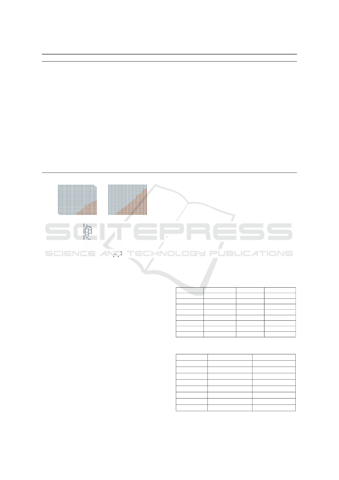
desired categorization of the input space. Consider
the example dataset with two classes in Figure 4c. In
this figure, one of the classes consists of only a few
instances, whereas the other class contains a larger
number of instances compared to the first one. With
the rule utilized in (Fawcett, 2008), the instance space
would be categorized into almost two equal size re-
gions as seen in Figure 4b. This bias introduced by
the method could be a serious drawback especially for
noisy data.
In Figure 4a, the same dataset is classified by us-
ing SCA-classification. The bias introduced by the
ICPRAM 2019 - 8th International Conference on Pattern Recognition Applications and Methods
158
Algorithm 3: The Overall Algorithm.
1: procedure SCA–CLASSIFY(CELLULAR AUTOMATON CA, DATASET D)
2: MAPDATA(CA,D
train
)
3: int continue=1
4: int iteration=0
5: while (continue) do
6: Cell C=getCellFromSelectionSet(CA)
7: HEAT–PROPAGATION(C)
8: Cell C=getCellFromSelectionSet(CA)
9: STATE–TRANSFER(C)
10: if iteration%1000 = 0 then
11: continue = ControlValidationPoints(CA,D
validation
)
12: end if
13: iteration++
14: end while
15: N ←− getNotAssignedClassList(CA, D
validation
)
16: for each cell K ∈ N do
17: DETERMINE–LABEL(K)
18: end for
19: end procedure
(a) (b)
(c)
Figure 4: Comparison of classification approaches: SCA-
classification(a), Manhattan distance classification(b), and
Data distribution(c).
heat transfer procedure in the algorithm enables the
denser class to spread to a larger area in the CA
compared to the other class consisting of only a few
elements. In (Fawcett, 2008), experimental results
are reported only on five real-world datasets and the
method is tested on datasets consisting of only 2
classes. We have the impression that the method is not
applicable to multi-class real-world datasets. There-
fore, we have decided to compare SCA-classification
with other state of the art classification methods, in-
stead of the approach presented in (Fawcett, 2008).
The next subsection firstly presents the description
of the datasets utilized in the experiments and then
a comparison between SCA-classification and some
other methods is presented.
3.1 SCA-classification on (UCI)
Datasets
Experiments are carried out on 8 different datasets
from UCI data repository (Newman and Merz, 1998).
Table 1 presents the properties of the datasets utilized
in the experiments. As seen in the table, datasets with
different number of attributes and classes are selected
for the experiments.
Correlation Based Feature Selection: method
(Hall and Smith, 1998) have been applied on the
datasets before the classification process in order to
Table 1: Datasets utilized in the experiments.
Dataset # of Attributes # of Classes # of Instances
Iris 2 3 150
Banknote 2 2 1372
Glass 8 7 214
Heart 7 2 270
Australian 5 2 690
Haberman 2 2 306
Pima 2 2 768
Breast-wisc 9 2 699
Table 2: Experimental results for SCA-classification.
Dataset Mean Success(%) Best Solution(%)
Iris 95.00 ± 3.07 100.0
Banknote 88.76 ± 1.92 93.09
Glass 50.47 ±6.50 65.12
Heart 78.15 ± 6.24 85.19
Australian 83.55 ± 3.04 89.13
Haberman 70.16 ± 4.03 75.81
Pima 69.68 ± 4.74 76.62
Breast-wisc 93.71 ± 2.36 97.86
A Cellular Automata based Classification Algorithm
159
reduce the dimensionality of the datasets. For the
Iris dataset, petal length and petal width, for the Ban-
knote dataset, 1
st
and 2
nd
attributes are selected by the
method. Only the Si attribute is removed in the reduc-
tion process for the Glass dataset. Heart dataset has 13
attributes orginally. 7 attributes are selected which are
chest, resting electrocardiographic result, maximum
heart rate archived, exercise induced angina, oldpeak,
number of major vessels and and thal. On the other
side, the number of attributes are reduced from 14 to
5 for the Australian dataset. The attributes chosen by
the method are the 5
th
, 8
th
, 10
th
, 13
rd
and 14
th
ones.
The attributes the year of operation and the number of
positive nodes are the selected ones for the Haberman
dataset. For Pima dataset, the plasma, body mass in-
dex, pedigree function and age attributes are selected.
Lastly, Breast-wisc dataset has 9 attributes originally.
No attribute is removed for this dataset in the attribute
reduction process. In Table 1, the remaining final
number of attributes are presented.
In Table 2, the performance of SCA-classification
is presented on the selected datasets. The results de-
note the accuracy on the test sets that are chosen ran-
domly. The average performance is the mean of 10
different runs. The result of the best run is also pre-
sented in the table.
In Table 5, effects of different threshold values
are denoted by conducting an experiments on the iris
data. Obviously, it requires more time when thresh-
old values are increased. Also, mean success slightly
decreases for higher threshold values.
In Table 3, a set of synthetic datasets generated by
Gaussian Generator (Handl, 2017) has been utilized
in order to unveil the effect of number of classes and
attributes on performace metrics: accuracy and run-
time. When the number of classes in 2-dimensional
datasets is steadily increased, accuracy decreases,
since data instances belonging to different classes be-
come closer. Also, runtime increases since the num-
ber of instances in the datasets increase with more
classes. On the other side, the number of attributes
do not have a significant effect on the metrics as seen
in the table.
Table 3: Analysis of SCA-classification on synthetic
datasets in terms of the number of clusters and attributes.
# of Attributes # of Classes Mean Success(%) Mean Runtime(s)
2 5 99.94±0.06 0.55
2 10 99.75±0.25 0.93
2 15 98.24±1.40 1.47
2 20 95.86±1.60 2.01
2 25 89.13±3.59 2.71
2 30 85.80±1.49 4.28
3 5 100.0±0.00 0.93
4 5 99.84±0.12 1.91
5 5 100.0±0.00 1.58
6 5 100.0±0.00 11.16
7 5 100.0±0.00 87.72
In Table 4, the accuracy obtained by different
classification methods on the same datasets is given.
The results are collected from a set of studies in
the literature and when a method is not applied to a
dataset, this is denoted as ”-” in the table. It is not
possible to claim that SCA-classification outperforms
other classification methods. However, we believe
that the results are promising and compatible with the
results in literature. For instance, SCA-classification
is better than Decision Table and ZeroR methods on
the Iris dataset and it has a slightly higher accuracy
compared to Decision Trees on Australian dataset.
An interesting result is that the method has a similar
performance with the Naive Bayes method on the
datasets except Haberman where Naive Bayes has a
better accuracy. The difference between the perfor-
mance of the two methods is always less than 5% on
the remaining datasets.
Note that a n-dimensional CA is needed for a
dataset consisting of n attributes. Therefore, the
number cells in the CA increases exponentially for
high dimensional datasets. In section 2.4, it has
been noted that a partial CA is utilized in order to
overcome this problem. The partial CA consists
of only the cells that have a data instance and their
neighbors at the beginning. However, as the heat
energy propagates in the automaton, new neighbor
cells are added to the partial CA. In order to analyze
the growth of the CA, three datasets are selected with
different number of attributes.
The first dataset is Iris which is a 2−dimensional
dataset. The second one is the Australian dataset
with five attributes. The last dataset chosen for the
analysis is Breast-wisc which has nine attributes. The
increase in the size of CA utilized is given in Figures
5a, 5b and 5c for these three datasets. As seen in
the figures, more cells are added to the initial CA
throughout the generations. However, the increase in
the total number of cells is almost linear for all of the
three datasets.
In order to analyze the performance of the pro-
posed method on big data, two additional datasets are
generated by Gaussian Generator (Handl, 2017). In
Table 6, the number of attributes and classes of these
two datasets are presented.
The performance comparison of SCA-
classification with some other algorithms is presented
in Table 8 and Table 7. The other classification
algorithms are tested on these datasets by using
the machine learning software WEKA(Witten
et al., 2016). The success rate obtained by SCA-
classification is compatible with the results obtained
by other classification methods. However, the
runtime performance of SCA-classification is not
ICPRAM 2019 - 8th International Conference on Pattern Recognition Applications and Methods
160
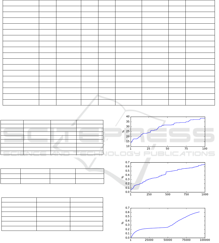
Table 4: Experimental results of other algorithms for the datasets are given in the table. References for each dataset are as
follows (Gupta, 2015), (Ghazvini et al., 2014),(Gupta, 2015),(Gupta, 2015),(Verma and Mehta, 2014),(Shruti and Khodanpur,
2015),(Parashar et al., 2014),(Shajahaan et al., 2013).
Method Iris Banknote Glass Heart Australian Haberman Pima Breast-wisc
Naive Bayes 96.00 88.04 47.66 75.36 85.20 76.47 - 97.42
Decision Tree - - - - 82.20 - - -
C4.5 - - - - - - - 95.57
SVM - - - - - 77.12 - -
Decision Table 92.67 - 68.22 85.07 - - - -
J48 96.00 - 68.69 85.79 - - - -
ID3 - - - - - - - 92.99
Boosting - - - - 82.20 - - -
Bagging - - - - 84.30 - - -
Random Forest 96.00 - 80.37 86.08 84.40 - - -
ZeroR 33.33 - 35.51 55.50 - - - -
MLP 96.00 95.81 65.88 85.79 - - - -
GP 96.00 - 66.82 87.10 - - - -
CART - - - - - - - 92.42
PLS-LDA - - - - - - 74.40 -
FMM - - - - - - 69.28 -
LDA-SVM - - - - - - 75.65 -
Table 5: Analysis of threshold values on iris dataset.
Threshold(°C) Mean Success(%) Best solution(%) Mean Runtime(s)
10 94.67±3.71 100.0 6.01
20 93.33±3.65 100.0 5.68
30 94.00±5.12 100.0 18.53
40 94.33±6.16 100.0 109.47
50 93.33±2.58 96.67 130.42
60 92.00±4.27 100.0 139.79
70 89.33±3.89 93.33 162.02
80 89.00±5.78 96.67 157.51
Table 6: The two big Datasets utilized.
Dataset # of Attributes # of Classes # of Instances
Dataset1 3 8 405419
Dataset2 5 8 48046
Table 7: Experimental results for Dataset1.
Method Mean Success(%) Mean Runtime(s)
SCA-classification 100.0 745.53 ± 9.19
Naive Bayes 100.0 3.20 ± 0.23
MLP 100.0 385.30 ± 5.54
ZeroR 14.61 ± 0.05 0.31± 0.35
Decision Table 99.99 ± 0.003 4.99 ± 0.34
Random Forest 100.0 69.58 ± 0.96
satisfactory compared to the fast classification algo-
rithms like Naive Bayes or Decision Tables. On the
first dataset SCA-classification has the lowest runtime
performance and on the second one only MultiLayer
Perceptrons have a worse performance compared to
SCA-classification. However, the method is open to
parallelization and as with Multilayer Perceptrons,
the runtime efficiency could be improved by parallel
execution.
(a) Iris dataset
(b) Australian dataset
(c) Breast-wisc dataset
Figure 5: Relation between the percentage of the cells cre-
ated in the CA(y-axis) and the number of iterations(x-axis).
4 CONCLUSION
In this paper, a novel approach based on CA is pro-
posed for the classification problem. The method has
A Cellular Automata based Classification Algorithm
161
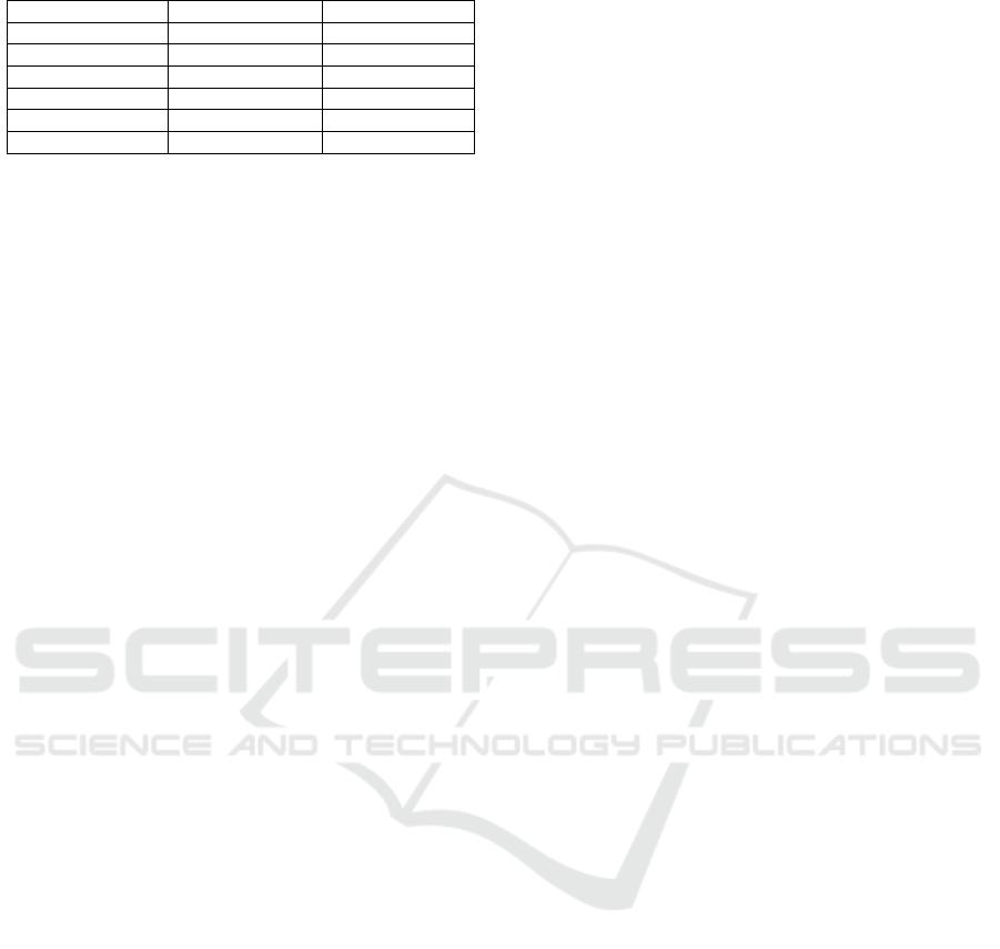
Table 8: Experimental results for Dataset2.
Method Mean Success(%) Mean Runtime(s)
SCA-classification 47.82 ± 1.52 40.14 ± 2.14
Naive Bayes 39.54 ± 0.47 0.28 ± 0.03
MLP 51.72 ± 1.05 53.21 ± 1.49
ZeroR 14.88 ± 0.19 0.03 ± 0.02
Decision Table 56.33 ± 0.57 3.53 ± 0.18
Random Forest 89.00 ± 0.12 20.50 ±0.25
an inductive bias inspired from the heat transfer pro-
cess in nature. The approach provides a framework
where cellular automata can be successfully used for
the classification process. The approach is tested on
datasets with different characteristics and promising
results have been obtained. Some future work can
be carried out to improve the algorithm. Firstly, the
CA utilized have equal number of cells in each di-
mension. Different number of cells can be chosen
in each dimension based on data characteristics. As
noted in the previous section, the method is also open
to parallelization which would improve the run-time
efficiency.
ACKNOWLEDGEMENTS
Enes Burak D
¨
undar contributed this study while he
was a student at Yeditepe University.
REFERENCES
Cheeseman, P., Self, M., Kelly, J., Taylor, W., Freeman, D.,
and Stutz, J. C. (1988). Bayesian classification. In
AAAI, volume 88, pages 607–611.
Cortes, C. and Vapnik, V. (1995). Support-vector networks.
Machine learning, 20(3):273–297.
D
¨
undar, E. B. and Korkmaz, E. E. (2018). Data cluster-
ing with stochastic cellular automata. Intelligent Data
Analysis, 22(3).
Ermentrout, G. B. and Edelstein-Keshet, L. (1993). Cellular
automata approaches to biological modeling. Journal
of theoretical Biology, 160(1):97–133.
Esmaeilpour, M., Naderifar, V., and Shukur, Z. (2012). Cel-
lular learning automata approach for data classifica-
tion. International Journal of Innovative Computing,
Information and Control, 8(12):8063–8076.
Fawcett, T. (2008). Data mining with cellular automata.
ACM SIGKDD Explorations Newsletter, 10(1):32–39.
Friedl, M. A. and Brodley, C. E. (1997). Decision tree clas-
sification of land cover from remotely sensed data. Re-
mote sensing of environment, 61(3):399–409.
Gardner, M. (1970). Mathematical games: The fantastic
combinations of john conway’s new solitaire game
“life”. Scientific American, 223(4):120–123.
Ghazvini, A., Awwalu, J., and Bakar, A. A. (2014). Com-
parative analysis of algorithms in supervised classifi-
cation: A case study of bank notes dataset. Computer
Trends and Technology, 17(1):39–43.
Gupta, A. (2015). Classification of complex uci datasets
using machine learning and evolutionary algorithms.
International journal of scientific and technology re-
search, 4(5):85–94.
Hall, M. A. and Smith, L. A. (1998). Practical feature subset
selection for machine learning.
Handl, J. (2017). Cluster generators. http://personalpages
.manchester.ac.uk/mbs/julia.handl/generators.html.
Accessed: 2017-12-19.
Hesselbarth, H. and G
¨
obel, I. (1991). Simulation of recrys-
tallization by cellular automata. Acta Metallurgica et
Materialia, 39(9):2135–2143.
Kokol, P., Povalej, P., Lenic, M., and Stiglic, G. (2004).
Building classifier cellular automata. In Sloot, P.
M. A., Chopard, B., and Hoekstra, A. G., editors,
ACRI, volume 3305 of Lecture Notes in Computer Sci-
ence, pages 823–830. Springer.
Langton, C. G. (1984). Self-reproduction in cellu-
lar automata. Physica D: Nonlinear Phenomena,
10(1):135–144.
Mai, J. and Von Niessen, W. (1992). A cellular automa-
ton model with diffusion for a surface reaction system.
Chemical physics, 165(1):57–63.
Margolus, N., Toffoli, T., and Vichniac, G. (1986). Cellular-
automata supercomputers for fluid-dynamics model-
ing. Physical Review Letters, 56(16):1694.
Newman, C. B. D. and Merz, C. (1998). UCI repository of
machine learning databases.
Parashar, A., Burse, K., and Rawat, K. (2014). A compara-
tive approach for pima indians diabetes diagnosis us-
ing lda-support vector machine and feed forward neu-
ral network. International Journal of Advanced Re-
search in Computer Science and Software Engineer-
ing, 4:378–383.
Povalej, P., Kokol, P., Dru
ˇ
zovec, T. W., and Stiglic, B.
(2005). Machine-learning with cellular automata. In
International Symposium on Intelligent Data Analy-
sis, pages 305–315. Springer.
Shajahaan, S. S., Shanthi, S., and ManoChitra, V. (2013).
Application of data mining techniques to model breast
cancer data. International Journal of Emerging Tech-
nology and Advanced Engineering, 3(11):362–369.
Shruti, A. and Khodanpur, B. (2015). Comparative study of
advanced classification methods. International Jour-
nal on Recent and Innovation Trends in Computing
and Communication, 3(3):1216–1220.
Uzun, A. O., Usta, T., D
¨
undar, E. B., and Korkmaz,
E. E. (2018). A solution to the classification problem
with cellular automata. Pattern Recognition Letters,
116:114 – 120.
Verma, M. and Mehta, D. (2014). A comparative study
of techniques in data mining. International Journal
of Emerging Technology and Advanced Engineering,
4(4):314–321.
Witten, I. H., Frank, E., Hall, M. A., and Pal, C. J. (2016).
Data Mining: Practical machine learning tools and
techniques. Morgan Kaufmann.
ICPRAM 2019 - 8th International Conference on Pattern Recognition Applications and Methods
162
