
Advances in Phase Retrieval by Transport of Intensity Equation
Dingfu Chen
1,2 a
, Anand Asundi
2,3 b
, Liansheng Sui
2,4 c
, Chongtian Huang
2,3 d
, Chi Wang
1
and
Yingjie Yu
1
1
Lab of Applied Optics and Metrology, Department of Precision Mechanical Engineering, Shanghai University,
Shanghai, China
2
Centre for Optical and Laser Engineering, School of Mechanical and Aerospace Engineering, Nanyang Technological
University, Singapore, Singapore
3
School of Computer Science and Engineering, Xi’an University of Technology, Xi’an, China
4
d’Optron Pte Ltd, Singapore, Singapore
Keywords: Transport of Intensity Equation, Transmission, Defocus Distance, Focus Plane, Magnification, High Order of
Intensity Derivatives.
Abstract: There are many factors in the calculations of Transport of Intensity Equation, which may lead to the
uncertainty of the retrieved phase. In this paper, effect of these parameters such as defocus distance, focus
plane and magnification, on the results is studied. It is hoped that this would provide a more robust and reliable
method for phase and optical height measurement. Furthermore, the effect of intensity derivatives calculated
using two defocussed images as opposed to multiple images is also considered. A microlens array is chosen
as the test sample in a commercial transmissive Transport of Intensity Equation system. From this study, it is
concluded that the biggest factor influencing the result is the magnification, which is seen to provided totally
different phase value for the same shape. Incorrect defocus distance or in-focus plane also lead to inaccurate
reconstruction results while higher order differential provides better and more stable results than traditional
two image differential.
1 INTRODUCTION
Quantitative phase imaging is finding diverse
application both in the precision measurement and
bio-medical imaging sectors. Non-interferometric
quantitative phase retrieval such as coherent
diffractive imaging (Williams et al., 2006) and
Transport of Intensity Equations (Teague, 1983)
provide greater flexibility in operation. Transport of
Intensity Equation (TIE) is a two-dimensional second
order elliptic differential equation proposed by
Teague (Roddier, 1988), which provides a
relationship between intensity and the phase of a light
wave in the near Fresnel regime. In the past few
decades, TIE has found a variety of applications in
adaptive optics (Nugent et al., 1996), X-ray
diffraction (Ishizuka and Allman, 2005), electron-
a
https://orcid.org/0000-0002-8242-0644
b
https://orcid.org/0000-0003-3835-4624
c
https://orcid.org/0000-0002-1771-1664
d
https://orcid.org/0000-0001-8081-7034
microscopy (Streibl, 1984) and optical quantitative
phase imaging (Zuo et al., 2013).
Basically, TIE needs at least three (under, in- and
over focus) images or a series of through-focus
intensity images (Nugent et al., 2011) (Soto and
Acosta, 2007) (Waller and Tian, 2010) (Gureyev and
Nugent, 1997). The in-focus intensity image contains
no phase information; however, the variation of its
intensity along the direction of propagation
introduces phase contrast. In fact, any imaging system
with a complex transfer function will provide some
phase contrast. These images can then be inverted to
quantitatively extract phase and amplitude.
For a paraxial beam propagating along the Z axis,
the complex amplitude of the object is
, where
is the
intensity and φ is the phase of the object wave. The
derivative of intensity along the beam propagation
168
Chen, D., Asundi, A., Sui, L., Huang, C., Wang, C. and Yu, Y.
Advances in Phase Retrieval by Transport of Intensity Equation.
DOI: 10.5220/0007374701680173
In Proceedings of the 7th International Conference on Photonics, Optics and Laser Technology (PHOTOPTICS 2019), pages 168-173
ISBN: 978-989-758-364-3
Copyright
c
2019 by SCITEPRESS – Science and Technology Publications, Lda. All rights reserved
direction, Z, contains phase information that can be
retrieved TIE. The general equation for TIE is
(Blanchard and Greenaway, 1999):
(1)
where
is the intensity in the focal plane. is
the wave number. φ(x,y) is the phase which needs to
be calculated.
denotes the gradient operator over
the propagation direction, z. Phase can be recovered
from a measurement of intensity derivative along the
optical axis and solving Eq. 1. The Fast Fourier
Transform (FFT) method is widely used for solving
the Poisson equations deduced from Eq. 1. If
is constant (i.e. a pure-phase object) and
is
continuous in a region with smooth boundaries, then
the solution of the TIE is unique. The right side of the
Eq. 1 can be rewritten as (Gorthi and Schonbrun,
2012) (Zuo et al., 2013) :
(2)
the partial derivative in the left the side can be
calculated in a finite difference manner as:
(3)
by recording two images spaced ±z on either side of
focus (Soto and Acosta, 2007). For magnified images,
the z at the object-plane is given as
.
Although a lot of researches have been done on
TIE, the retrieval phase results still have some
uncertainties based on the choice of to obtain the
derivative. A shorter would approximate the
derivative better but will be influenced by noise,
while a larger would smooth the result but would
not be an accurate representative of the gradient. As
in finite difference approaches, a series of images can
be used to take advantage of the two cases. This paper
would consider this and other effects such as
magnification in the determination of phase.
2 EXPERIMENTAL SYSTEM
C. Zuo et al introduced an image relay system (Zuo et
al., 2013) to replace the traditional mechanical
translation of camera to record the out of focus
images. This was commercialized by d’Optron Pte ltd
(www.doptron.com) and has been applied for
biological and industrial quantitative phase imaging.
The system can be configured for both transmission
and reflection measurement. It can be used as a stand-
alone system or can be adapted onto any microscope
for increased spatial resolution. The axial resolution
of the system is in the order of tens of nm. Figure 1
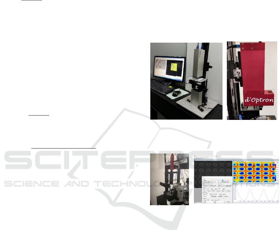
shows both the transmission and reflection stand-
alone system, while Figure 2(a) shows the system as
adapted to a microscope. The system has its own
software shown in Figure 2(b) which allows the user
to manipulate the defocus planes as well as record a
series of images as desired. It also has the capability
of getting depth from focus for samples with large
depths.
(a)
(b)
Figure 1: Stand-alone d’Nanoimager systems for (a)
transparent samples and (b) reflecting samples.
Figure 2: (a) d’Nanoimager adapted to a microscope. (b)
Software interface.
3 EXPERIMENTAL SYSTEM
For this study, the d’Nanoimager is coupled to the
conventional Olympus BX41 transmission
microscope. A microlens array is measured using this
system. The size of the microlens array is
10mm10mm. The lens pitch is 75 . The software
allows a large number of images and different focus
distances to be rapidly recorded. Figure 3 shows a
sample of over 100 through focus images. Three such
image stacks were recorded using the same setup at
different magnification of 10 , 20 , 40 ,
respectively which could be analysed in a variety of
ways.
Advances in Phase Retrieval by Transport of Intensity Equation
169
(a)
(b)
(c)
(d)
(e)
(f)
Figure 3: A series of through focus intensity images at 20
magnification of a microlens array.
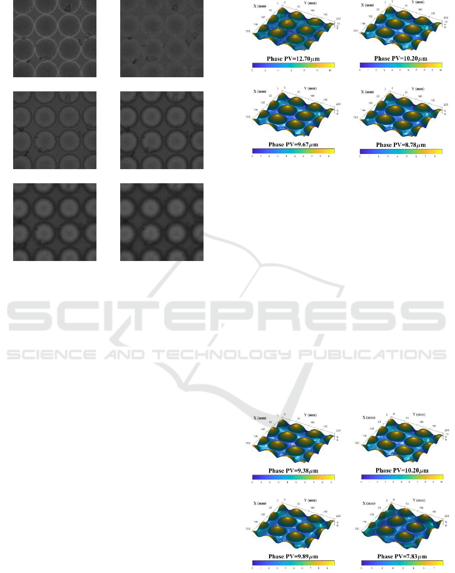
3.1 Effect of Defocus Distance
As observed earlier, when is large, the finite
difference approximation breaks down while for
smaller leads to increased noise. Images at different
defocus distances ranging from 0.8 to 23.0 μm
were chosen from the stack with the 25
th
image (Figure
3(b)) being the in-focus image. As expected, when the
defocus distance is small (Figure 4 (a)), the
reconstruction was noisy which smoothed as the
defocus distance increased (Figure 4(b)). However, the
image tends to blur as the defocus distance increases.
3.2 Effect of Focus Plane
The influence of choice of in-focus image,
, on the
experiment results is considered next. To verify this,
from the above image stack different in-focus image
planes are selected. To avoid effects of , the defocus
distance was set to 7.7 , which was the optimal
distance as per Section 3.1. Different in-focus planes
ranging from the bottom to the top of microlens were
selected from the same stack as earlier. As seen in
Figure 5, changes in the in-focus image plane leads to
a few changes in reconstructed phase. The phases in
Figure 5(a-c) looks quite similar but their height values
are different. While in Figure 5(d) where the in-focus
(a)
(b)
(c)
(d)
Figure 4: Phase retrieval using different defocus distance.
(a) =0.8 . (b) =7.7 . (c) =15.3 . (d)
=23.0 .
plane was on top of the microlens, the phase does not
accurately describe the shape of an object.
To clearly highlight the effects of in-focus image
and defocus distance, line plots of retrieved phase as
function of the in-focus image plane are plotted as
shown in Figure 6 for different defocus distance. As the
number of images in the stack are fixed a larger
defocus distance means fewer focus planes are
available. So, the green line is the shortest and the blue
line is the longest. It is interesting to note that the peak
shifts to the right for increasing defocus distance and
there is a reduction in the Peak to Valley (P-V) value,
indicating smoothing of the result. Also, if the in-focus
image is chosen at the wrong plane, the defocus images
do not contain the entire information of the surface of
the microlens array, resulting in lower phase values.
(a)
(b)
(c)
(d)
Figure 5: Phase retrieval with different in-focus image
plane. (a) Focus at the background of microlens 20
th
(b)
focus at the bottom of microlens 30
th
. (c) focus at the 50
th
plane. (d). focus at the 80
th
plane of microlens.
PHOTOPTICS 2019 - 7th International Conference on Photonics, Optics and Laser Technology
170
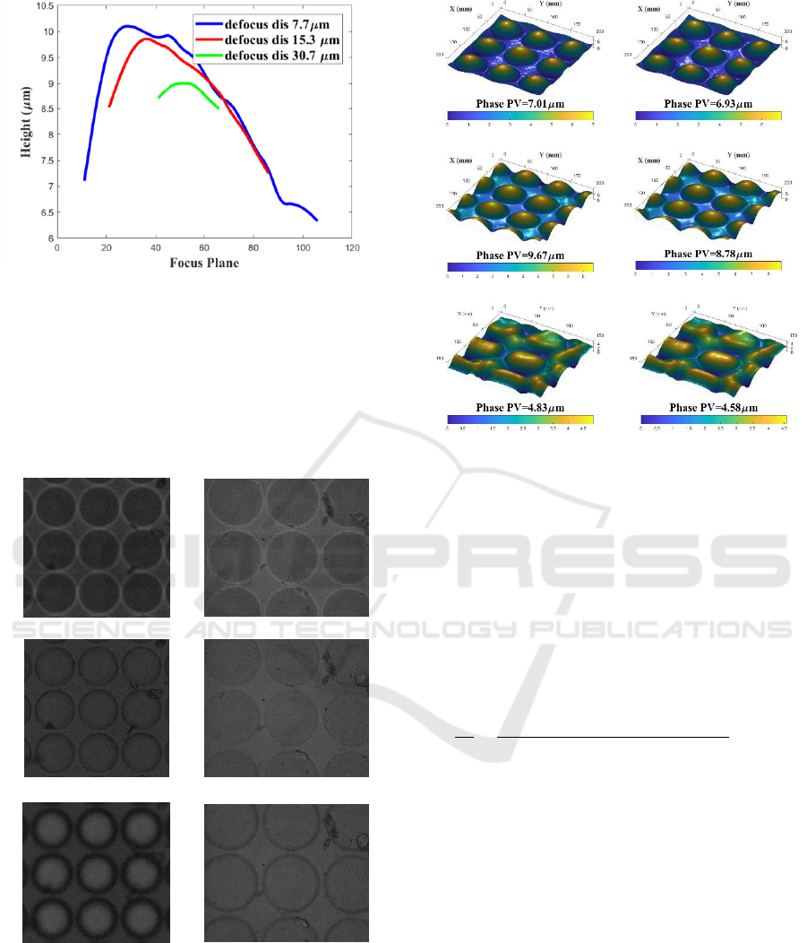
Figure 6: Effect of in-focus image and the defocus distance.
3.3 Effect of Magnification
For this hypothesis, experiments were conducted at
10, 20, 40 magnification. Figure 7 shows typical
recorded intensity images. Due to the magnification,
the at the object plane for a 40 system is 6.2 ,
smaller than the height of the microlens.
(a)
(b)
(c)
(d)
(e)
(f)
Figure 7: Intensity images of 10 magnification. (a) -26
under-focus image. (c) in-focus image. (e) +26
over-focus. Intensity images of 40 magnification with
defocus distance (b) -3.10 (d) focus image. (f) +3.10
.
(a)
(b)
(c)
(d)
(e)
(f)
Figure 8: Phase retrieval of different magnification. (a) 10
, =15.7 (b) 10, =26 (c) 20, =7.7 .
(d) 20, =15.3 . (e) 40, =5.0 . (f) 40,
=9.9 .
3.4 Effect of Multiple Defocus Images
Waller (Soto and Acosta, 2007) demonstrated a
method for improving the accuracy of phase retrieval
based on TIE by using multiple images to estimate the
derivative:
(4)
where
is the image weighting,
is the intensity
image at , with
as the focused image,
negative n corresponds to under focus images, and
positive n corresponds to over focus images. So, 2n+1
is the total number of the images and is the order of
the derivatives.
In this step, we chose two groups of data - at 10
and 20 magnification. For the 20 dataset, 3, 7 and
15 images with defocus distances of 7.7 , 0.77
and 0.77 respectively and the in-focus image
being the 30th image in the stack were selected.
Figure 9(a-c) shows that the results are very close. For
the 10 dataset, 7 and 15 images with a 2.67
defocus distance was tested with the in-focus image
being the 30
th
image in the stack. Figure 9(d, e) shows
consistent results. In order to clearly see the
difference between the phase retrieved by 7 and 15
Advances in Phase Retrieval by Transport of Intensity Equation
171
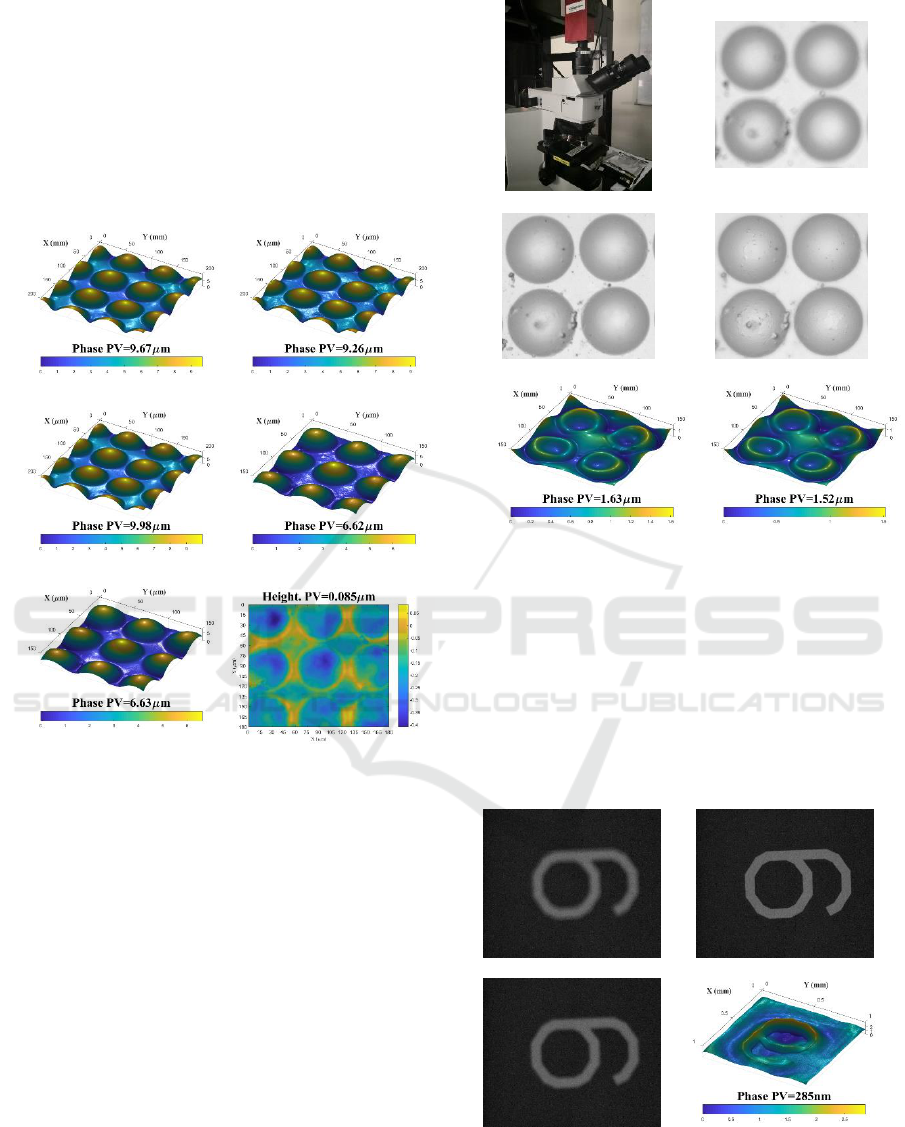
images, the difference of Figure 9(d) and Figure 9(e)
show a PV deviation of 0.085.
Higher order TIE results show better quality than
the lower order ones. However, too many images also
blur the phase. The traditional TIE with 3 images is
hidden behind low frequency noise and artifacts,
while the retrieval phase with 15 images leads to the
nonlinear error. Using 7 images seems to be a good
compromise.
(a)
(b)
(c)
(d)
(e)
(f)
Figure 9: Phase retrieval using (a) 3 images, 20, =7.7
focus at the 30
th
plane. (b) 7 images, 20, =0.383
focus at the 30
th
plane. (c) 15 images, 20, =0.767
focus at the 30
th
plane. (d) 7 images, 10, =2.67
focus at the 30
th
plane. (e) 15 images, 10, =2.67
focus at the 30
th
planes. (f) the deviation between (d) and
(e).
3.5 Effect of Reflective TIE
Transmissive TIE will be affected by the phase of the
bottom surface which may also affect the final phase
calculation. The d’Nanoimager is coupled to a
Olympus reflective microscope at 10 magnification
as shown in Figure 10(a), to measure top surface only.
Figures 10(b-d) show typical recorded intensity
images at different planes. As can be seen, due to the
curvature of the lens, the top part appears to be too
bright which would affect the calculation. The dust on
the surface of the microlens array, helped identify the
50
th
image as the in-focus image.
(a)
(b)
(c)
(d)
(e)
(f)
Figure 10: a serial of intensity images with reflective
microscope. (a) d’Nanoimager adapted to a reflective
microscope. (b) -15.7 under-focus image. (c) in-focus
image. (d) 15.7 over-focus image. (e) the retrieved phase.
(f) the retrieved phase with 23.6 μm defocus distance.
From the Figure 10(e, f), it is observed that the
central part results are not correct – which could be
due to the over-saturation of intensity resulting in
little or no variation between the different images.
(a)
(b)
(c)
(d)
Figure 11: Intensity images with reflective microscope. (a)
-163 under-focus image. (b) the in-focus image. (c) 163
over-focus image. (d) the retrieved phase using 31
images.
PHOTOPTICS 2019 - 7th International Conference on Photonics, Optics and Laser Technology
172

To confirm this a USAF target is also chosen as a
sample to be measured with 5 magnification (Figure
11). Since the image was noisy, 31 terms were used
to calculate the intensity derivative. between the
adjacent image is 10.8 . The result shows the good
performance of the TIE, except for the sharp
boundary points.
4 CONCLUSIONS
In this paper, the effect of different parameters on the
retrieved phase by TIE method is explored. Using the
commercial system from d’Optron, image stacks can
be quickly collected. The greatest impact was from
the magnification effect, which caused the largest
change in the measured height. Other aspects of the
magnification need to be further studied. Besides, the
effect of the defocus distance and the choice of the in-
focus plane also affects the result. We must ensure
that the three images must span the entire height of
the surface, otherwise, the retrieved phase is
incorrect. Furthermore, using more terms to calculate
the derivative can get more stable result. However,
excessive number of images will offset the impact of
noise and smooth the phase. About 7 images appears
to be an optimal number. The reflective setup would
be affected by large intensity variations especially if
the curvature of the surface is large, however for
flatter object such as the USAF target the results are
quite good.
ACKNOWLEDGEMENTS
The authors acknowledge the support from the
National Natural Science Foundation of China
(NSFC) Project No. 51775326 and the National
Science and Technology Major project No.
2016YFF0101805.
REFERENCES
Williams, G. J., Quiney, H. M., Dhal, B. B., Tran, C. Q.,
Nugent, K. A., Peele, A. G., Paterson, D., Jonge, M. D.,
2006. Fresnel Coherent Diffractive Imaging. Phys. Rev.
Lett. 97(2), 025506.
Teague, M. R., 1983. Deterministic phase retrieval: a
Green's function solution. J. Opt. Soc. Am. 73(11),
1434–1441.
Roddier, F., 1988. Curvature sensing and compensation: a
new concept in adaptive optics. Appl. Opt. 27(7), 1223–
1225
Nugent, K. A., Gureyev, T. E., Cookson, D. J., Paganin, D.,
Barnea, Z., 1996. Quantitative phase imaging using
hard X rays. Phys. Rev. Lett. 77(14), 2961–2964
Ishizuka, K., Allman, B., 2005 Phase measurement of
atomic resolution image using transport of intensity
equation. J. Electron Micros. 54(3), 191–197.
Streibl, N., 1984. Phase imaging by the transport equation
of intensity, Opt. Comm. 49(1), 6–10.
Zuo, C., Chen, Q., Qu, W. J., Asundi, A., 2013.
Noninterferometric single-shot quantitative phase
microscopy. Opt. Letter. 38(18), 3538–3541.
Nugent, K., Paganin, D., Gureyev, T., 2001. A phase
odyssey. Physics Today 54, 27–32.
Soto, M., Acosta, E., 2007. Improved phase imaging from
intensity measurements in multiple planes. Appl. Opt.
46, 7978–7981.
Waller, L., Tian, L., Barbastathis, G., 2010. Transport of
intensity phase-amplitude imaging with higher order
intensity derivatives. Opt. Express. 18, 12552–12561
Gureyev, T., Nugent, K., 1997. Rapid quantitative phase
imaging using the transport of intensity equation. Opt.
Comm. 133(1-6), 339–346.
Blanchard, P. M., Greenaway, A. H., 1999. Simultaneous
multiplane imaging with a distorted diffraction grating.
Appl. Opt. 38, 6692–6699.
Gorthi, S. S., Schonbrun, E., 2012. Phase imaging flow
cytometry using a focus-stack collecting microscope.
Opt. Lett. 37, 707–709.
Zuo, C., Chen, Q., Qu, W., Asundi, A., 2013. High-speed
transport of -intensity phase microscopy with an
electrically tunable lens. Opt. Express. 21(20), 24060-
24075.
d’Nanoimager by d’Optron Pte Ltd., www.doptron.com.
Advances in Phase Retrieval by Transport of Intensity Equation
173
