
Annealing by Increasing Resampling
in the Unified View of Simulated Annealing
Yasunobu Imamura
1
, Naoya Higuchi
1
, Takeshi Shinohara
1
, Kouichi Hirata
1
and Tetsuji Kuboyama
2
1
Kyushu Institute of Technology, Kawazu 680-4, Iizuka 820-8502, Japan
2
Gakushuin University, Mejiro 1-5-1, Toshima, Tokyo 171-8588, Japan
Keywords:
Annealing by Increasing Resampling, Simulated Annealing, Logit, Probit, Meta-heuristics, Optimization.
Abstract:
Annealing by Increasing Resampling (AIR) is a stochastic hill-climbing optimization by resampling with
increasing size for evaluating an objective function. In this paper, we introduce a unified view of the con-
ventional Simulated Annealing (SA) and AIR. In this view, we generalize both SA and AIR to a stochastic
hill-climbing for objective functions with stochastic fluctuations, i.e., logit and probit, respectively. Since the
logit function is approximated by the probit function, we show that AIR is regarded as an approximation of
SA. The experimental results on sparse pivot selection and annealing-based clustering also support that AIR
is an approximation of SA. Moreover, when an objective function requires a large number of samples, AIR is
much faster than SA without sacrificing the quality of the results.
1 INTRODUCTION
The similarity search is an important task for informa-
tion retrieval in high-dimensional data space. Dimen-
sionality reduction such as SIMPLE-MAP (Shinohara
and Ishizaka, 2002) and Sketch (Dong et al., 2008) is
known to be one of the effective approaches for effi-
cient indexing and fast searching. In dimensionality
reduction, we have to select a small number of axes
with low distortion from the original space. This op-
timal selection gives rise to a hard combinatorial op-
timization problem.
Simulated annealing (SA) (Kirkpatrick and
Gelatt Jr., 1983) is known to be one of the most
successful methods for solving combinatorial op-
timization problems. It is a metaheuristic search
method to find an approximation optimal value
of an objective function. Initially, SA starts with
high temperature, and moves in the wide range of
search space by random walk. Then, by cooling the
temperature slowly, it narrows the range of search
space so that finally it achieves the global optimum.
On the other hand, we present a method called an
annealing by increasing resampling (AIR), which is
introduced originally for the sparse pivot selection for
SIMPLE-MAP as a hill-climbing algorithm by resam-
pling with increasing the sample size and by evaluat-
ing pivots in every resampling (Imamura et al., 2017).
AIR is suitable to optimization problems that sam-
pling is used due to the computational costs, and the
value of the objective function is given by the aver-
age of evaluations for each sample. For example, in
the pivot selection problem (Bustos et al., 2001), the
objective function is given by the average of the pair-
wise distances in the pivot space for each set of sam-
ples, and pivots are selected such that they maximize
the average.
In the processes near the initial stage of the AIR,
the sample size is small and then the local optimal is
not stable and moving drastically because the AIR re-
places the previous sample with an independent sam-
ple by resampling. On the other hand, in the processes
near the ending stage of the AIR, the sample size is in-
creasing and then the local optimal is stable. This pro-
cess of AIR is similar to conventional hill-climbing
algorithms. The larger the sample size grows, the
smaller the error in the evaluation becomes. At the
final stage, AIR works like a local search as SA. In
other words, AIR realizes behavior like SA. In addi-
tion, AIR is superior to SA on its computational costs
especially when the sample size for evaluating objec-
tive functions are very large, because AIR uses small
set of samples near the initial stage for which the eval-
uation can be done in very short time.
In the previous work (Imamura et al., 2017), we
introduce AIR for a specific problem, pivot selection.
In this paper, we show that AIR is applicable as a
more general optimization method through the unified
Imamura, Y., Higuchi, N., Shinohara, T., Hirata, K. and Kuboyama, T.
Annealing by Increasing Resampling in the Unified View of Simulated Annealing.
DOI: 10.5220/0007380701730180
In Proceedings of the 8th International Conference on Pattern Recognition Applications and Methods (ICPRAM 2019), pages 173-180
ISBN: 978-989-758-351-3
Copyright
c
2019 by SCITEPRESS – Science and Technology Publications, Lda. All rights reserved
173

view of SA and AIR. In the view, both methods are
formed as a hill-climbing algorithm using a objective
function with stochastic fluctuation. The fluctuation
of the evaluation in SA using acceptance rate by Hast-
ings (Hastings, 1970) can be explained by logit, and
that of AIR can be explained with probit. Since logit
can be approximated by probit, AIR can be viewed as
an approximation of SA.
The experimental results show that the global op-
timum in SA requires a large amount of computation
while cooling the temperature. On the other hand,
for AIR, increasing the size of sample for evaluating
an objective function corresponds to cooling the tem-
perature in SA. Hence, AIR can efficiently search the
global optimum with realizing the large number of it-
erations by increasing resampling instead of cooling
the temperature in SA without sacrificing the quality
of the solution.
Furthermore, we give comparative experiments
by applying SA and AIR to two optimization prob-
lems, the sparse pivot selection for dimensional-
ity reduction using SIMPLE-MAP (Shinohara and
Ishizaka, 2002) and the annealing-based clustering
problem (Merendino and Celebi, 2013). The results
show that AIR is an approximation of SA, and AIR is
much faster than SA when the sample size for evalu-
ation is very large.
2 UNIFIED VIEW OF SA AND AIR
In this section, we give a unified view between the
simulated annealing (SA) (Kirkpatrick and Gelatt Jr.,
1983) and the annealing by increasing resampling
(AIR) (Imamura et al., 2017). The notations used are
shown in Table 1. Here, we consider the minimizing
problem of objective (energy) function E : U ×S →R,
where U is the solution space, that is, the set of all
possible solutions), and S is the sample dataset. The
goal is to find a global minimum solution x
∗
such that
E(x
∗
,S) ≤ E(x,S) for all x ∈ U. We also use the no-
tation E(x) if the dataset S is used for evaluating ob-
jective function, i.e., E(x) = E(x,S).
2.1 Simulated Annealing
In SA, we call the procedure to allow for occasional
changes that worsen the next state an acceptance
probability (function) (Anily and Federgruen, 1987)
or acceptance criterion (Schuur, 1997). For the ac-
ceptance probability P, Algorithm 1 illustrates the
general schema for SA.
There are two acceptance probabilities com-
monly used in SA. One is a Metropolis function
Table 1: Notations.
Notation Description
t ∈ N time steps (0,1,2,. ..)
T
t
≥ 0 temperature at t
(monotonically decreasing)
S dataset for evaluating objective func-
tion E
s(t) ∈ N resampling size at t ≤ |S|
(monotonically increasing)
U solution space
x,x
0
∈U elements of solution space U
N(x) ⊆U neighborhood of x ∈U
E(x, S
0
) evaluation value for x ∈ U and dataset
S
0
⊆ S
procedure SA
// T
t
: the temperature at t
// S: sample data for evaluation
// rand(0,1): uniform random number
// in [0,1)
x ← initial state;
for t = 1 to ∞ do
x
0
←
randomly selected state from N(x);
∆E ← E(x
0
) −E(x);
ω ← rand(0,1);
if ω ≤ P(T
t
) then x ← x
0
;
Algorithm 1: Simulated annealing.
P
M
(Metropolis et al., 1953), which is a standard
and original choice in SA (Kirkpatrick and Gelatt Jr.,
1983).
P
M
(T ) = min{1,exp(−∆E/T )}.
Another is a Barker function (Barker, 1965) (or a heat
bath function (Anily and Federgruen, 1987)) P
B
as a
special case of a Hastings function (Hastings, 1970),
which has been introduced in the context of Boltz-
mann machine (Aarts and Korst, 1989).
P
B
(T ) =
1
1 + exp(∆E/T )
.
Consider the condition that x
0
is selected in N(x)
after x is selected. For the Metropolis function P
M
, it
holds that ω ≤ exp(−∆E/T
t
), which implies that
∆E + T
t
·log(ω) ≤ 0.
For the Barker function P
B
, it holds that
ω ≤
1
1 + exp(∆E/T
t
)
,
which implies that exp(∆E/T
t
) ≤
1−ω
ω
and then
∆E + T
t
·logit(ω) ≤ 0, (1)
ICPRAM 2019 - 8th International Conference on Pattern Recognition Applications and Methods
174

where logit(·) is the logit function defined as
logit(ω) = −log
1 −ω
ω
.
Now, we are to minimize the value of E(·,·). Hence,
if ∆E is less than zero, we want to transit to a “bet-
ter” state x
0
. The left-hand side of the acceptance con-
dition Eq. (1) is considered as ∆E with disturbance
proportional to temperature T
t
.
In SA, the temperature is gradually cooled down
to avoid getting trapped in a local minimum. On the
other hand, AIR uses the sample size of data instead
of temperature.
2.2 Annealing by Increasing
Resampling
In AIR, we consider the objective function for sam-
ple S
0
from dataset S , and the problem of minimizing
the average of evaluation values for samplings from
S. AIR is an optimization method taking advantage
of the nature that the smaller the sampling size is, the
larger the fluctuation of evaluation is. Algorithm 2
illustrates the procedure of AIR.
procedure AIR
// T
t
: temperature at t
// S: sample data
x ← initial state;
for t = 1 to ∞ do
x
0
←
randomly selected state from N(x);
S
0
←
randomly selected dataset from S
such that S
0
⊆ S and |S
0
| = s(t);
if E(x
0
,S
0
) −E(x,S
0
) ≤ 0 then x ← x
0
;
Algorithm 2: Annealing by increasing resampling (AIR).
Let N = |S|, and assume that the difference be-
tween E(x, S
0
) and E(x
0
,S
0
) follows a normal distri-
bution with standard derivation σ. This assumption
is reasonable due to the central limit theory because
the objective function is obtained by the average of
evaluations for each set of independent samples.
Then, for samples S
0
of S such that |S
0
| = n, the
difference between E(x,S
0
) and E(x
0
,S
0
) also fol-
lows a normal distribution with the standard error.
In other words, E(x
0
,S
0
) − E(x,S
0
) is the value of
E(x
0
,S) −E(x, S) with fluctuation of standard deriva-
tion
σ
√
n
·
q
N−n
N−1
, where the term
q
N−n
N−1
is the finite
population correlation factor of
σ
√
n
. Hence, for a uni-
formly random variable ω ranging from 0 to 1, it holds
that
E(x
0
,S
0
) −E(x,S
0
) (2)
= E(x
0
,S) −E(x,S) +
σ
√
n
·
r
N −n
N −1
·probit(ω),
where probit(·) is the inverse of the cumulative dis-
tribution function of the standard normal distribution.
Note that probit(ω) follows the normal distribution if
ω follows the uniformly random distribution between
0 and 1.
In AIR, since a subsample S
0
of S is selected by
resampling, the next subsample of S needs to be se-
lected independently from S
0
. As a similar approach,
we incrementally add a small number of samples from
S to S
0
without replacement. This approach allows
us a faster computation since we can reuse the previ-
ous computation for the current evaluation of sample
S
0
. However, we do not employ this approach in AIR
since the stochastic trials on the selection of state x
0
at
each time needs to be made independently. It is nec-
essary to independently select a subsample for each
trial, but to improve the efficiency of the process, the
current subsample may be reused, but sometimes the
subsample must be replaced.
2.3 General View of Annealing-based
Algorithms
Now we confirm that the acceptance criterion of SA
based on Hasting function is
∆E + T
t
·logit(ω) ≤ 0, (3)
where ∆E = E(x
0
) − E(x), and note that E(x) =
E(x, S) if S is the dataset with maximum size to use.
In contrast, the acceptance criterion of AIR is
∆E +
σ
√
n
·
r
N −n
N −1
·probit(ω) ≤ 0. (4)
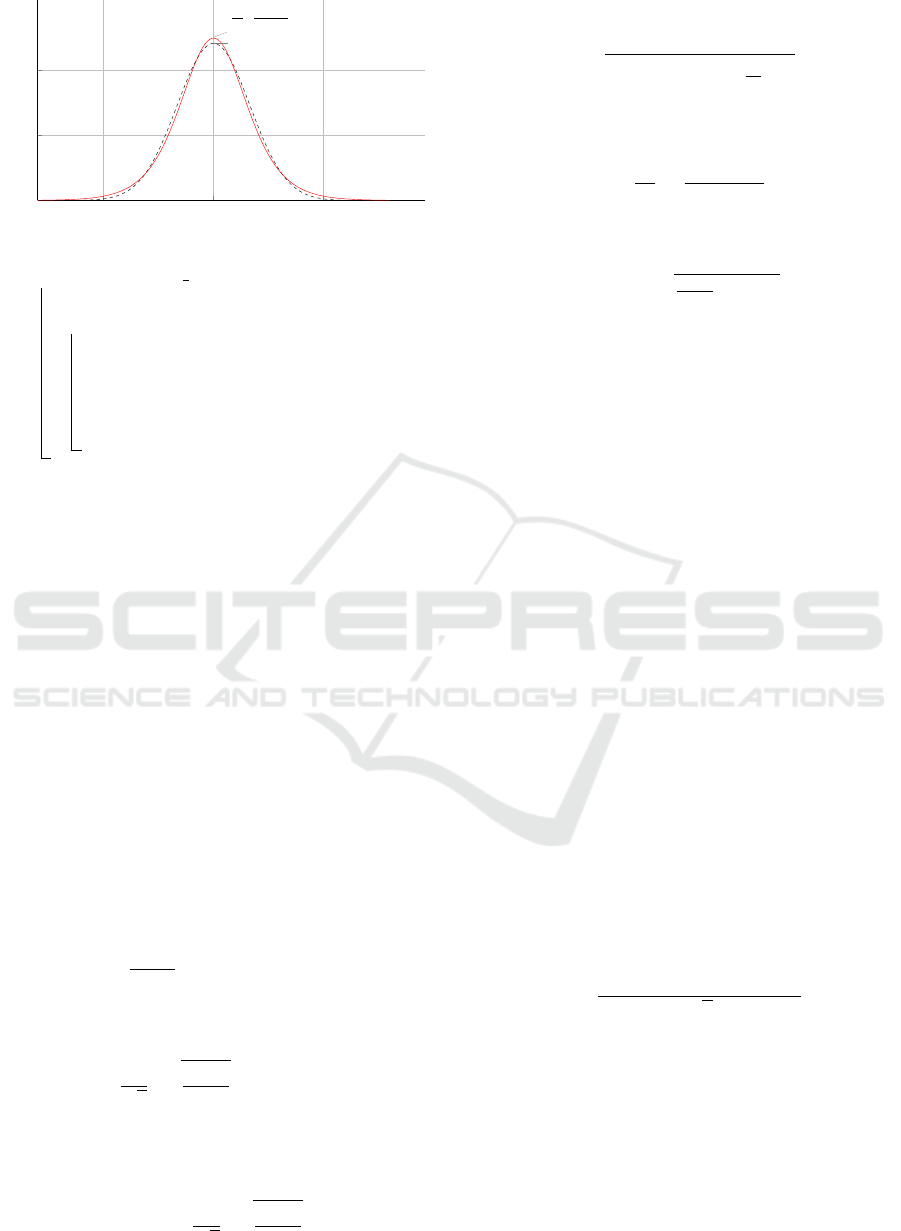
Both criteria Eq. (3) and Eq. (4) are in the same
form. Also, it is known that the normal distribu-
tion is approximated by the logistic distribution; i.e.
logit(ω) ≈ σ
0
·probit(ω) when σ
0
= 1.65 as shown in
Figure 1 (Demidenko, 2013).
Therefore, we can generalize the acceptance crite-
rion of SA and AIR as follows.
∆E + α(t)·Φ
−1
(ω) ≤ 0, (5)
where α(·) is a monotonically decreasing function for
time step t (note that the dataset size n is given by
the function s(t) in AIR), and Φ
−1
(·) is the inverse of
the cumulative distribution function of a probability
distribution. Algorithm 3 shows the unified procedure
of SA and AIR.
Annealing by Increasing Resampling in the Unified View of Simulated Annealing
175
−5 0 5
0.1
0.2
d
dx
1
1 + e
−x
N (0, 1.65)
Figure 1: Logistic distribution and normal distribution.
procedure Unified Annealing
x ← initial state;
for t = 1 to ∞ do
x
0
←
randomly selected state from N(x);
ω ← rand(0,1);
if E(x
0
) −E(x) +α(t) ·Φ
−1
(ω) ≤ 0
then x ← x
0
;
Algorithm 3: Unified procedure of SA and AIR.
2.4 Annealing Schedules of SA and AIR
The temperature cooling schedule is an important fac-
tor of SA for efficiency and accuracy. We consider the
corresponding sample size schedule in AIR to the ex-
ponential cooling scheme in SA. Here, we define the
schedule as follows.
T = T
0
·T
r
(0 < T
r
< 1),
where T
0
,T , and T
r
is the initial temperature, the cur-
rent temperature, and the ratio between T and T
0
, re-
spectively; Note that T
r
monotonically decreases as
the value of t increases. Let N, n
0
and n be the maxi-
mum sample size, the initial sample size, and the cur-
rent sample size, respectively. Also, let σ
0
be approx-
imately 1.65, and σ the standard deviation per sample.
The acceptance criterion of the next state x
0
in SA
is given by
∆E + T ·log
ω
1 −ω
= ∆E + T ·logit(ω) ≤ 0. (6)
On the other hand, the acceptance criterion in AIR is
given by
∆E +
σ
√
n
·
r
N −n
N −1
·probit(ω) ≤ 0. (7)
Since logit(ω) ≈ σ
0
·probit(ω) (Demidenko, 2013),
in order to equate formulae Eq. (6) and Eq.(7), it is
sufficient to satisfy the following condition.
T ·σ
0
=
σ
√
n
·
r
N −n
N −1
.
It follows that
n =
N
(N −1) ·T
2
0
·T
2
r
·
σ
2
0
σ
2
+ 1
.
By noting that T
r
= 1 and n = n
0
when T = T
0
, it holds
that
T
2
0
·
σ
2
0
σ
2
=
N −n
0
(N −1)n
0
.
Hence, we have
s(t) = n =
N
N−n
0
n
0
·T
2
r
+ 1
. (8)
The sample size n at time step t is given by the
function of t. Note that s(0) = n
0
. This for-
mula bridges the relationship between the tempera-
ture cooling scheduling T = T
0
·T
r
in SA and the sam-
ple size scheduling in AIR. By using the same ratio T
r
between SA and AIR, we can consider that two ap-
proaches are fairly compared in the experiments.
3 EXPERIMENTAL RESULTS
3.1 AIR Approximated by SA
In this experiment, we consider how much AIR is
approximate to SA by using MCMC (Markov chain
Monte Calro method for Metropolis-Hastings algo-
rithm), which is the basis of SA. We use MCMC in-
stead of optimization for evaluating the accuracy be-
cause it is necessary to evaluate the accuracy of distri-
bution estimation of the objective function regardless
of scheduling.
We employ the correlation coefficient ρ as the ap-
proximation accuracy between the estimated distribu-
tion and the actual distribution with sampling points,
and the approximation error as 1 −ρ. A simple one-
dimensional function shown below is used as the ob-
jective function (this function itself is not essential).
y =
0.3e
−(x−1)
2
+ 0.7e
−(x+2)
2
√
π
.
This objective function is the mixture of two normal
distributions with two maxima. Experiments are con-
ducted in the following six acceptance criteria:
1. Metropolis Acceptance Criterion:
ω ≤ min{1,exp(−∆E/T
t
)}.
2. Hastings Acceptance Criterion:
ω ≤ min{1,exp(−∆E/T
t
)}.
ICPRAM 2019 - 8th International Conference on Pattern Recognition Applications and Methods
176
3. Φ
−1
(ω) = log(ω):
∆E + T
t
·log(ω) ≤ 0.
4. Φ
−1
(ω) = logit(ω):
∆E + T
t
·logit(ω) ≤ 0.
5. Φ
−1
(ω) = 1.60 ·probit(ω):
∆E + T
t
·1.60 ·probit(ω) ≤ 0.
6. Φ
−1
(ω) = 1.65 ·probit(ω):
∆E + T
t
·1.65 ·probit(ω) ≤ 0.
As shown in Section 2.1, the criterion (1) is equiv-
alent to the criterion (3), and the criterion (2) is to
the criterion (4) theoretically. The criteria (5) and (6)
correspond to the acceptance criteria in AIR which
approximate Hastings acceptance criterion by setting
σ = 1.60 and σ = 1.65, respectively as stated in the
condition of Eq. (4).
10
5
10
6
10
7
10
8
10
−5
10
−4
10
−3
10
−2
Number of Transitions
Estimation Error
1. Metropolis
2. Hastings
3. log(ω)
4. logit(ω)
5. 1.60 ·probit(ω)
6. 1.65 ·probit(ω)
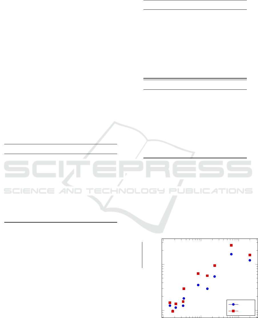
Figure 2: Estimation errors in MCMC with six acceptance
criteria.
In the experimental setting, we discard the initial
10
5
transitions as the burn-in phase. Then, we evalu-
ate the estimation errors with 1000 discrete points of
correlation coefficients. Each estimation is carried out
ten times, and the average is taken as the estimation.
Figure 2 shows the estimation errors for each criteria
obtained by the experiment.
Due to the theoretical correspondences, the esti-
mation error of (1) Metropolis and (3) log(ω), and
that of (2) Heistings and (4) logit(ω) are almost
identical, respectively. As for the criteria (5) 1.60 ·
probit(ω) and (6) 1.65 ·probit(ω), up to the number
of transitions of 10
6
, it is observed that both are good
approximations of SA with Hastings acceptance cri-
terion. Although, beyond 10
7
transitions, a signif-
icant difference appears as shown in Figure 2, it is
not a concern since the number of transitions at each
temperature is less than 10
7
in real computations of
AIR. Also, it is not necessary to care about the op-
timal value of σ
0
because the temperature T absorbs
the effect of σ, and the optimal value of σ
0
is implic-
itly computed in practice.
3.2 Sparse Pivot Selection
We apply AIR to the sparse pivot selection for di-
mensionality reduction using SIMPLE-MAP (Shino-
hara and Ishizaka, 2002). We use real image data for
the pivot selection. In the dimension reduction, we
project data points in a high-dimensional space into a
lower dimensional space. The number of pivots in
SIMPLE-MAP corresponds to the dimensionality of
the projected space. It is required to select a small
number of pivots so that all pairwise distances be-
tween data points are preserved as much as possible
after projection. We call this problem sparse pivot se-
lection. The number of data in images is 6.8 million
extracted from 1,700 videos and dimensionality n of
data in images is 64. In this experiment, we reduce the
number of dimensions to eight using SIMPLE-MAP.
We use the average value (Ave.) and the standard de-
viation (S.D.) for distance preservation ratio (DPR)
to evaluate pivot sets using randomly selected 5,000
pairs of features. AIR finds the set of pivots with max-
imum distance preservation ratio. We set the compat-
ible annealing schedule between SA and AIR accord-
ing to Eq. (8). The experimental platform is a 64-bit
mac OS X machine with 2.53GHz Intel
R
Core
TM
i5
and 8GB RAM.
Table 2: Comparison SA with AIR in pivot selection.
DPR(%)
#transitions Time (sec) Ave. S.D.
SA 11 ×10
3
149.7 57.06% 0.2763
40 ×10
3
511.1 57.36% 0.2379
400 ×10
3
4864.0 57.52% 0.1485
AIR 11 ×10
3
28.80 57.10% 0.2260
40 ×10
3
70.49 57.36% 0.1333
400 ×10
3
592.5 57.57% 0.1547
Table 2 shows the results for each number of tran-
sitions. The best value for each performence measure
is highlighted in bold face. Note that a larger the aver-
age value for DPR implies, a better result. This exper-
iment shows that AIR achieves almost the same accu-
racy with much faster speeds (from 5.2 to 8.2 times
faster) than SA.
Annealing by Increasing Resampling in the Unified View of Simulated Annealing
177
3.3 Annealing-based Clustering
In this experiment, we focus on a clustering method
using SA. The typical objective function to minimize
is the sum of squared errors (SSE) between each point
and the closest cluster center.
Merendino and Celebi proposed an SA clustering
algorithm based on center perturbation using Gaus-
sian mutation (SAGM, for short) (Merendino and
Celebi, 2013). SAGM employs two cooling sched-
ules, the multi Markov chain (MMC) approach, and
the single Markov chain (SMC) approach. We denote
SAGM with MMC schedule by SAGM(MMC), and
SAGM with SMC schedule by SAGM(SMC). They
reported that SAGM(SMC) generally converges sig-
nificantly faster than the other SA algorithms with-
out losing the quality of solutions as comparison with
the others through the experiments using ten datasets
from the UCI Machine Learning Repository (Dheeru
and Karra Taniskidou, 2017). Table 3 shows the de-
scription of the datasets used in the experiments.
Table 3: Datasets (N: #points, d: #attributes, k: #classes).
ID Data Set N d k
1 Ecoli 336 7 8
2 Glass 214 9 6
3 Ionosphere 351 34 2
4 Iris Bezdek 150 4 3
5 Landsat 6435 36 6
6 Letter Recognition 20000 16 26
7 Image Segmentation 2310 19 7
8 Vehicle Silhouettes 846 18 4
9 Wine Quality 178 13 7
10 Yeast 1484 8 10
We implement both SAGM(MMC) and
SAGM(SMC) in C++, and AIR with the corre-
sponding schedulings MMC and SMC according
to Eq. (8), denoted by AIR(MMC) and AIR(SMC),
respectively. Then, we compare the quality of
solutions and the running time for the datasets. The
experiments are conducted with an Intel
R
Core
TM
i7-
7820X CPU 3.60Hz, and 64G RAM, running Ubuntu
(Windows Subsystem for Linux) on Windows 10.
The quality of the solutions is evaluated by SSE.
Then, a smaller SSE implies a better result.
Table 4 shows the quality of solutions (SSE) with
the standard deviations in parenthesis by comparing
SAGM(MMC) with AIR(MMC) in the upper table,
and by comparing SAGM(SMC) with AIR(SMC) in
the lower table. It is confirmed that there is no sig-
nificant differences between SAGM and AIR in the
quality of solutions.
Table 5 shows the running time for both SAGM
Table 4: Quality of solutions (Sum of squared errors).
Data ID SAGM(MMC) AIR(MMC)
1 17.55 (0.23) 17.53 (0.20)
2 18.91 (0.69) 19.05 (0.45)
3 630.9 (19.76) 638.8 (43.42)
4 6.988 (0.03) 6.986 (0.02)
5 1742 (0.01) 1742 (0.01)
6 2732 (14.17) 2720 (4.20)
7 411.9 (18.11) 395.2 (10.68)
8 225.7 (4.54) 224.6 (3.82)
9 37.83 (0.23) 37.81 (0.23)
10 58.90 (1.65) 59.08 (0.74)
Data ID SAGM(SMC) AIR(SMC)
1 17.60 (0.29) 17.56 (0.24)
2 18.98 (0.73) 19.08 (0.46)
3 630.9 (19.76) 646.8 (57.14)
4 6.988 (0.03) 6.991 (0.03)
5 1742 (0.01) 1742 (0.01)
6 2738 (17.11) 2722 (5.10)
7 413.8 (19.88) 396.2 (11.26)
8 225.8 (4.65) 224.6 (3.83)
9 37.85 (0.27) 37.82 (0.24)
10 59.36 (1.61) 59.04 (0.67)
and AIR. AIR is significantly faster than SAGM for
all datasets except for the 9th dataset in both schedul-
ing MMC and SMC. For the 9th dataset, SAGM
slightly outperforms AIR because the size of the
dataset is very small (n = 178).
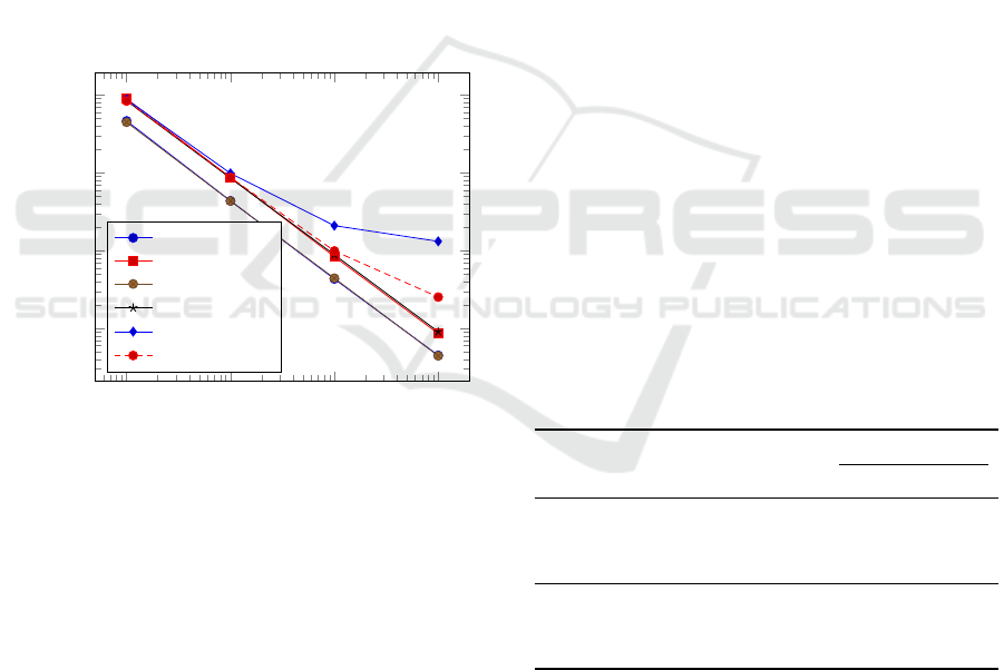
To observe the effect of the data size N on the
running time, Figure 3 show the running time ratios
of SAGM to AIR for each scheduling of MMC and
SMC. As can be seen from the figure, the larger the
data size is, basically the faster AIR is, and the sam-
pling effect of AIR appears.
10
2
10
3
10
4
10
0
10
1
Data size (N)
Running time ratios (
SAGM[sec]
AIR[sec]
)
MMC
SMC
Figure 3: Runnning time ratios of SAGM to AIR.
ICPRAM 2019 - 8th International Conference on Pattern Recognition Applications and Methods
178

Table 5: Average running time (sec.).
Data ID SAGM(MMC) AIR(MMC)
1 1.727 1.376
2 0.719 0.629
3 1.549 0.857
4 0.139 0.110
5 17.40 1.051
6 167.4 13.72
7 3.285 0.606
8 1.298 0.367
9 0.786 0.814
10 2.854 0.971
Data ID SAGM(SMC) AIR(SMC)
1 0.282 0.182
2 0.125 0.091
3 0.281 0.095
4 0.022 0.015
5 3.216 0.125
6 28.82 1.803
7 0.523 0.056
8 0.219 0.035
9 0.141 0.149
10 0.497 0.088
4 CONCLUSIONS
A sampling-based meta heuristics method, Annealing
by Increasing Resampling (AIR), is a stochastic hill-
climbing optimization by resampling with increasing
size for evaluating an objective function. It uses the
resampling size n instead of temperature T in the sim-
ulated annealing (SA). We showed a unified view of
SA and AIR by the approximation of logit and probit
in the hill-climbing algorithm.
We also showed the relationship between sample
size n in AIR and temperature T in SA from the the-
oretical point of view. Since the resampling size n
exponentially increases up to the total sample size N
when a common resampling size scheduling is em-
ployed. Hence, the size n is not affected by N un-
til the final step. This is the reason why AIR is
much faster than the conventional SA especially for
the large dataset.
We also conducted experiments to support our
view, and showed that AIR achieves almost the same
quality of solutions with much faster computation
than SA by applying AIR to the sparse pivot selection
problem and the clustering problem.
The superiority of AIR over SA is that the compu-
tational cost for transitions using small sample sets,
corresponding to transisions in the high temperature
of SA, is small. For actual problems, a stable opti-
mization by SA is necessary to increase the number
of transitions at the high temperature. Even in such
cases, when using AIR, it is possible to improve the
performance of optimization without increasing the
cost much. The scheduling that takes advantage of the
benefits of AIR is one of the important future works.
Another important future work is the implementa-
tion of efficient similarity search in high dimensional
spaces using dimensionality reductions and sketches
highly optimized by AIR.
ACKNOWLEDGMENTS
The authors would like to thank Prof. M. Emre
Celebi who kindly provides us with the source codes
of SAGM with both SMC and MMC schedules.
This work was partially supported by JSPS
KAKENHI Grant Numbers 16H02870, 17H00762,
16H01743, 17H01788, and 18K11443.
The first author would like to thank several pro-
gramming contests because providing the motivation
of this paper. In many problms in the contests, pa-
rameter tuning plays a crucial role for efficient com-
putations and he actually has applied AIR to the au-
tomated parameter tuning in programming contests,
and remarkable achievements have been made so far
by AIR.
REFERENCES
Aarts, E. and Korst, J. (1989). Simulated annealing and
Boltzmann machines: A stochastic approach to com-
binatorial optimization and neural computing. Wiley.
Anily, S. and Federgruen, A. (1987). Simulated anneal-
ing methods with general acceptance probabilities.
J. App. Prob., 24:657–667.
Barker, A. A. (1965). Monte Carlo calculations of the radial
distribution functions for a proton-electron plasma.
Aust. J. Phys., 18:119–133.
Bustos, B., Navarro, G., and Ch
´
avez, E. (2001). Pivot se-
lection techniques for proximity searching in metric
spaces. In Proc. Computer Science Society. SCCC’01.
XXI Internatinal Conference of the Chilean, pages 33–
40. IEEE.
Demidenko, E. (2013). Mixed Models: Theory and Appli-
cations with R. Wiley, 2nd edition.
Dheeru, D. and Karra Taniskidou, E. (2017). UCI ma-
chine learning repository. University of California,
Irvine, School of Information and Computer Sciences,
http://archive.ics.uci.edu/ml.
Dong, W., Charikar, M., and Li, K. (2008). Asymmetric
distance estimation with sketches for similarity search
Annealing by Increasing Resampling in the Unified View of Simulated Annealing
179

in high-dimensional spaces. In Proc. 31st ACM SIGIR,
pages 123–130.
Hastings, W. K. (1970). Monte Carlo sampling methods
using Markov chains and their applications. Biome-
toroka, 57:97–109.
Imamura, Y., Higuchi, N., Kuboyama, T., Hirata, K., and
Shinohara, T. (2017). Pivot selection for dimension
reduction using annealing by increasing resampling.
In Proc. Learn. Wissen. Daten. Analysen, (LWDA’17),
pages 15–24.
Kirkpatrick, S. and Gelatt Jr., C. D. (1983). Optimization
by simulated annealing. Science, 220:671–680.
Merendino, S. and Celebi, M. E. (2013). A simulated an-
nealing clustering algorithm based on center perturba-
tion using Gaussian mutation. In Proc. FLAIRS Con-
ference, pages 456–461.
Metropolis, N., Rosenbluth, A. W., Rosenbluth, M. N., and
Teller, A. H. (1953). Equation of state calculations by
fast computing machines. J. Chem. Phys., 21:1086–
1092.
Schuur, P. C. (1997). Classification of acceptance
criteria for the simulated annealing algorithm.
Math. Oper. Res., 22:266–275.
Shinohara, T. and Ishizaka, H. (2002). On dimension re-
duction mappings for approximate retrieval of multi-
dimensional data. In Arikawa, S. and Shinohara, A.,
editors, Progress in Discovery Science, volume 2281
of LNCS, pages 224–231. Springer.
ICPRAM 2019 - 8th International Conference on Pattern Recognition Applications and Methods
180
