A Content-aware Filtering for RGBD Faces

Leandro Dihl

, Leandro Cruz

, Nuno Monteiro

and Nuno Gonc¸alves

1,3

Institute of Systems and Robotics, University of Coimbra, Portugal

Institute for Systems and Robotics, University of Lisbon, Portugal

Portuguese Mint and Ofﬁcial Printing Ofﬁce, Portugal

Keywords:

Mesh Geometry Model, Mesh Denoising, Filtering.

Abstract:

3D face models are widely used for several purposes, such as biometric systems, face veriﬁcation, facial ex-

pression recognition, 3D visualization, and so on. They can be captured by using different kinds of devices,

like plenoptic cameras, structured light cameras, time of ﬂight, among others. Nevertheless, the models gener-

ated by all these consumer devices are quite noisy. In this work, we present a content-aware ﬁltering for 2.5D

meshes of faces that preserves their intrinsic features. This ﬁlter consists on an exemplar-based neighborhood

matching where all models are in a frontal position avoiding rotation and perspective. We take advantage of

prior knowledge of the models (faces) to improve the comparison. We ﬁrst detect facial feature points, create

the point correctors for regions of each feature, and only use the correspondent regions for correcting a point

of the ﬁltered mesh. The model is invariant to depth translation and scale. The proposed method is evaluated

on a public 3D face dataset with different levels of noise. The results show that the method is able to remove

noise without smoothing the sharp features of the face.

1 INTRODUCTION

The current advances of consumer RGBD cameras,

such as light ﬁelds cameras (Lytro (Ng et al., 2005)

and Raytrix (GmbH, 2018)), structured light cameras

(Kinect V1 (Microsoft, 2018)), time of ﬂight cameras

(Kinect V2 and Depth Sense (Sony, 2018)) and stereo

cameras (ZED (Stereolabs, 2018)) has allowed the re-

covering of geometric information of a scene. On one

hand, these consumer cameras are cheap and easily

available. On other hand, despite the wide range of

possible applications, the obtained geometry can be

very noisy and contains holes. Our work intends to

improve the geometric model obtained by any RGBD

camera for a speciﬁc context, namely faces. This ﬁl-

ter can be used to improve the input model of many

systems based on an RGBD facial model, for exam-

ple: face recognition, facial expression recovery and

pose detection. The goal of this work is: given a tar-

get facial model containing the texture, geometry (a

set of the X, Y, Z points arranged in a grid or a list)

and the respective texture mapping, we want to ob-

tain an RGBD model of the face whose geometry (Z)

is properly ﬁltered.

The proposed ﬁltering method assumes that the

geometric points are regularly arranged. This ﬁlter is

based on a statistical prediction process that modiﬁes

each point of the target mesh by comparing its neigh-

borhood with others of the same size from a model

whose geometry is considered appropriate (no noise,

without holes or other spurious artifacts). We denom-

inate this other model by exemplar.

The ﬁltering process assumes that both target and

exemplar are on the same scale and sampling fre-

quency (and then, a set of k × k z-values of target

can be compared to the same size set on exemplar).

However, in general, this is not the case for models

captured by different systems (device + reconstruc-

tion algorithm). Hence, in this work, we will also

present an approach to create an RGBD representa-

tion of the target in the same sampling frequency of

the exemplar.

In this way, the proposed approach begins with

data acquisition, which can be performed using any of

the aforementioned devices, followed by the respec-

tive reconstruction method. A full revision of recon-

struction methods is beyond the scope of this work.

We will keep focus on resampling of a point cloud or

a grid of points containing the geometry XYZ, texture

mapping UV and the texture RGB. After the acquisi-

tion, standardize the target (obtain a regular RGBD

model in the same sampling frequency of the exem-

270

Dihl, L., Cruz, L., Monteiro, N. and Gonçalves, N.

A Content-aware Filtering for RGBD Faces.

DOI: 10.5220/0007384702700277

In Proceedings of the 14th International Joint Conference on Computer Vision, Imaging and Computer Graphics Theory and Applications (VISIGRAPP 2019), pages 270-277

ISBN: 978-989-758-354-4

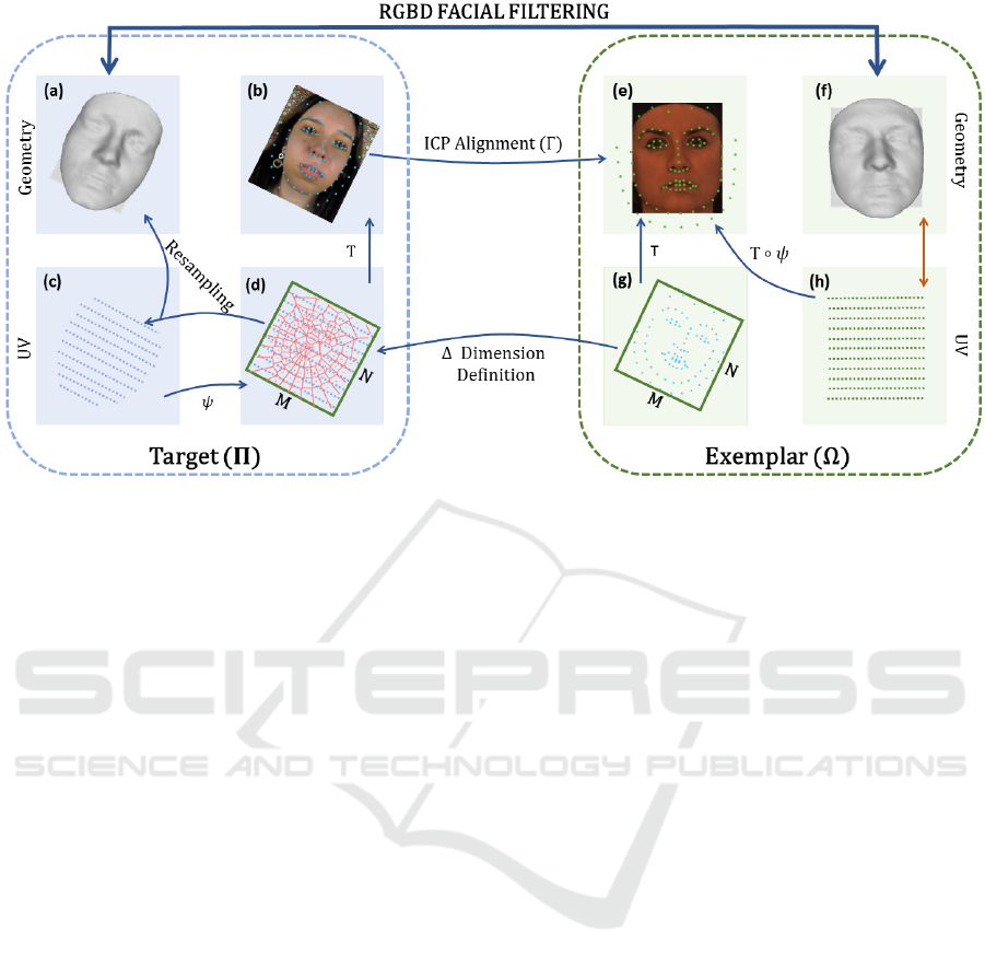
Figure 1: This Figure shows the taxonomy of our method. On the left, it is represented a target Π and its spaces (geometry

(a), texture (b, d) and UV (c)). On the right, it is represented an exemplar Ω, also with its spaces (geometry (f), texture (e, g)

and UV (h)).

plar). It will be explained in Section 3. In Section 4,

we will provide a description of our exemplar-based

ﬁltering method. Finally, in Section 5, we will present

the results and some conclusions.

2 RELATED WORK

In the last years, various ﬁltering approaches have

been proposed to process mesh geometry, denoising

and smoothing meshes aiming the output from 3D

scanners or 3D cameras. The image processing litera-

ture considers that methods of mesh denoising can be

classiﬁed in isotropic or anisotropic (Wei et al., 2018).

Isotropic methods are independent of surface ge-

ometry, they normally remove noise and high fre-

quency features together, for example, low-pass ﬁl-

ters were some of the ﬁrst proposed models to treat

meshes. These ﬁlters remove high-frequency noises

but also attenuate sharp features. (Taubin, 1995)

and (Desbrun et al., 1999). Thus, isotropic meth-

ods have difﬁculty in preserving geometric features.

Anisotropic ﬁlters are based on anisotropic geomet-

ric diffusion, which are inspired by scale space and

anisotropic diffusion in image processing (Perona and

Malik, 1990). They are often needed to preserve fea-

tures such as sharp edges and corners.

Yagou et al. (Yagou et al., 2002) modiﬁed to the

normal vector of a triangle according to the nor-

mal vectors of its neighbors and then updated the

vertices positions. Liu et al. (Liu et al., 2018)

introduced a new mesh ﬁltering method which is

calculated along the geodesic paths. Intrinsically,

through the integral of property differences along the

geodesic paths, weights calculated between neighbor-

ing faces are much more reliable. Lu and Deng (Lu

et al., 2016) presented a scheme for robust feature-

preserving mesh denoising. Given a noisy mesh input,

their method ﬁrst estimates an initial mesh, then per-

forms feature detection, identiﬁcation, and connec-

tion, and ﬁnally, iteratively updates vertex positions

based on the constructed feature edges. However, ac-

cording to the authors the approach present problems

in the noisy models with an extreme triangulation or

high levels of noise.

The works proposed by [(Botsch et al.,

2007), (Cho et al., 2014)] also perform mesh

denoising by ﬁltering the face normals, using a

general formulation of the bilateral ﬁlter with some

variants. Due to its simplicity and feature-preserving

capability, the bilateral ﬁlter has been used in count-

less applications in image processing. Zheng et al.

(Zheng et al., 2011) employed the bilateral ﬁlter to

the mesh face normals, then the process of vertex

updated is implemented according to the ﬁltered

normals. The effectiveness of various bilateral ﬁlters

mainly relies on the weight of measuring the range

differences.

The aforementioned approaches are based on a lo-

cal geometric neighbor information. If the noise level

is extremely high or if there is not enough informa-

tion due to acquisition problems, the approaches tend

to fail or produce undesired results.

A Content-aware Filtering for RGBD Faces

271

Our main objective is to present a robust ﬁlter-

ing model that keeps the information coherent and

reliable even if under the worst situations. This cor-

rection process is similar to that which is solved in

texture-based synthesis techniques (Wei et al., 2009).

Different from texture synthesis, our method has

prior knowledge about face structure. A face has

some particular properties, thus it is important the

ﬁltering keeps them in order to not defeaturing the

model. Although the model and exemplars have dif-

ferent macro-features (for instance, one can be larger

or lengthier than the other), it is possible to ob-

tain a matching of local features because respective

parts still have intrinsic geometric similarities. The

pipeline is illustrated in Figure 4.

3 MODEL STANDARDIZING

Distinct acquisition processes can result in models

with different scales and sampling frequencies. In

this section, we will present how to standardize a face

model.

This work is a content-aware ﬁltering for face

models. It can be adapted for other types of models

whether it has a way to relate a pair of captured mod-

els from different devices. A general relation between

two devices for generic model acquisition is beyond

the scope of this work. However, it may be performed

by calibrating the camera (by using speciﬁc patterns,

such as a chess pattern) that allows to relate model

measures, and then, guarantee the same sampling fre-

quency. It is important to highlight that our content-

aware approach does not require any calibration step,

it is performed by Facial Feature Points (FFP) (Wang

et al., 2018) matching.

The standardizing model process consists of

changing of frequency sampling of a given model,

named target Π, according to a base model, named

exemplar Ω. This exemplar is ﬁltering basis. In cases

when we use more than one exemplar to deﬁne the

ﬁlter, one of them is chosen to be the base, and the

others are also resampled.

The standardizing is performed in two main steps:

(i) the target-exemplar FFP alignment and (ii) the tar-

get resampling. They can be seen in the Figure (Fig-

ure 1). In Section 3.1, we will present the FFP deﬁ-

nition, and the target-exemplar alignment will be pre-

sented in Section 3.2. Following, we can deﬁne the

proper model resolution and then perform the resam-

pling. It will be presented in Section 3.3. The correc-

tion of the scale is performed on predictor deﬁnition,

that will be explained in Section 4.1.

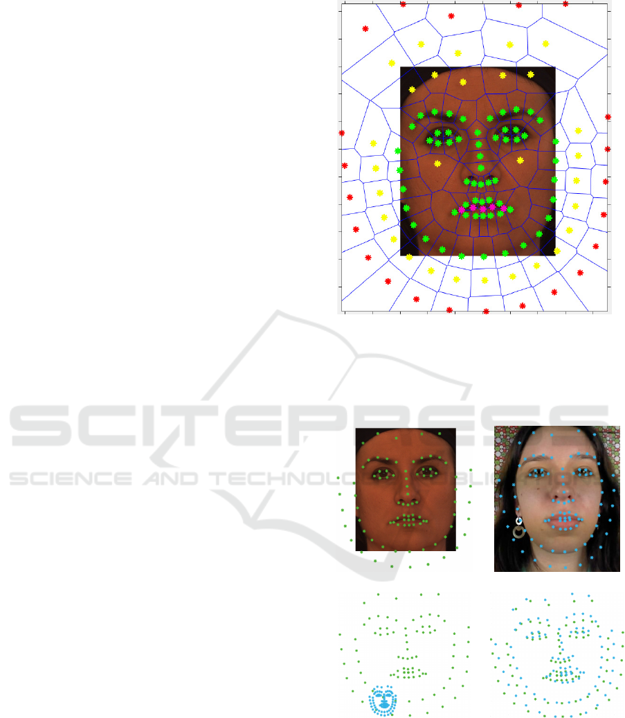
Figure 2: This Figure shows the initial detected FFPs,

(green points). The new points that are inserted (yellow

points) to split regions that does not satisfy the condition

(3) (forehead and cheeks) or to cover facial part that does

not reached by initial points. Unnecessary points (magenta

points) that are deleted. And, the red points that are inserted

to bound the external FFPs regions.

(a) (b)

Figure 3: This Figure shows the Facial Feature Points from

exemplar (a) and target (b). (c) shows the FFPs before

alignment and (d) the FFPs after alignment.

3.1 Facial Feature Points (FFPs)

The model standardizing is based on set minutiae

named Facial Feature Points (FFPs). These points

GRAPP 2019 - 14th International Conference on Computer Graphics Theory and Applications

272

are also known as facial landmarks, facial ﬁducial

points and Facial minutiae. They have a semantic

meaning: located around eyes, mouth, nose, chin, and

along face silhouette (Wang et al., 2018). They are

shown in Figure 3 (a) and (b). The generation of these

points is composed of the following steps: (i) detec-

tion, (ii) insertion, and (iii) removal of unnecessary

FFPs. In Section 4.1, we will explain (iv) how to cre-

ate the region of each FFP, based on Voronoi diagram

of these points (Aurenhammer, 1991), and ﬁnally ex-

plain (v) how to deﬁne the respective points of each

region. It goes without saying that this further steps

are performed on geometry space, hence the FFPs

have to be projected into this space (Figure 1(a)).

For a proper ﬁltering, it is important guarantee a

homogeneity of each FFP region. For this purpose,

the facial covering process shall meet three condi-

tions:

1. All faces must have FFP at correspondent places;

2. The union of regions must cover the whole face;

3. The area of each region must be inversely propor-

tional to the average of expected noise.

These conditions are achieved by an extension

of the set of FFPs proposed by Kazemi and Sulli-

van (Kazemi and Sullivan, 2014). This face detec-

tor uses Histogram of Oriented Gradients (HOG) fea-

ture combined with a linear classiﬁer, a pyramid im-

age, and sliding window detection scheme. After the

points detection, (Green points in the Figure 2), new

points are inserted (i) (Yellow points in the Figure 2)

to split regions that do not satisfy the condition (3).

For example, we added points on the center of the

cheeks and the forehead. These points are generated

between the eyes corners and project them from eye-

brows on the forehead. The cheek points are the cen-

tral points of the two lines created between the mouth

corners and the eyebrows corners, respectively. Fol-

lowing, unnecessary points are removed (ii) (Magenta

points in the Figure 2). It happens in areas where two

neighbor FFPs are often too close, such as the cen-

tral contour of the lips. The red points are inserted to

bound the external FFPs regions.

3.2 Target-exemplar FFP Alignment

Figure 1 shows all elements of these processing. A

model is composed of a list or a grid of points con-

taining the geometry (X,Y,Z)), the texture (an RGB

image) and the UV mapping (a function ψ that asso-

ciates each mesh point to the coordinates of the tex-

ture image).

The alignment of two models starts by deﬁn-

ing the FFP on respective texture. Next, the tar-

get FFPs (Figure 1 (b)) are aligned to the exemplar

FFPs (Figure 1 (e)) by using Iterative Closest Point

(ICP) (Zhang, 1994). This method returns a scale

s ∈ R, a rotation R (2 × 2 matrix), and a translation

c ∈ R

that, when applied over the Π FFPs, align

them to Ω FFPs in such a way that minimizes the

difference between the two point sets. It is an afﬁne

transformation that can be represented in homoge-

neous coordinates (adding for each point a third co-

ordinate equals to 1) by the following matrix:

Γ =





c.x

c.y

0 0 1





3×3

(1)

This afﬁne transformation can be visualized in

Figure1. After the alignment, we can perform the tar-

get resampling.

3.3 Target Resampling

The original target is a set Π = {P

, ..., P

} where we

have P

, y

, z

, u

, v

), that can be a point cloud or a

grid. Without loss of generality, we will assume it

as a point cloud. Additionally, it is provided an im-

age T (which dimension is W × H) that is the tex-

ture of this model. The texture mapping of a point

is given by a function ψ(p) = (p

.u ∗W, p

.v ∗ H).

It returns the pixel index of T related to p

, i.e. the

color of p

is T (ψ(p)). On the other hand, if ( j, i) are

the coordinates of a given point in the texture, then

(u, v) = ψ

−1

( j, i) = (

). Figure 1(g,h) illustrates

this mapping.

The resampling process consists of creating

a rectangular grid of target points, named ∆ =

{(x

, y

, z

, u

, v

);k = 1..M, l = 1..N}. It is per-

formed by the deﬁnition of the coordinates XYZ and

UV of M × N points (∆ dimension) taken regularly

into the target texture space (Figure 1 (g) to (d)). The

resampling is based on a triangulation of points of Π

in UV space.

The deﬁnition of M and N (∆ dimension) is based

on the target FFPs transformed into the exemplar

texture space. Each target FFP (into target texture

space) is multiplied on homogeneous coordinates by

Γ. It is created an oriented bounding box around these

transformed points. Finally, M and N are the dimen-

sions of this box.

Once deﬁned these dimensions, we have to cre-

ate the M × N points of ∆. The resampling starts

on texture (samples inside the face bounding box

in target texture space) and for each sample, we

have to deﬁne the respective XYZ and UV coor-

dinates. It is also needed to deﬁne ( j, i) for each

sample into target texture space, then the respective

A Content-aware Filtering for RGBD Faces

273

Figure 4: The pipeline of the ﬁltering method.

(u, v) = ψ

−1

( j, i). The coordinates (x, y, z) are ob-

tained based on this (u, v). We create a Delaunay

triangulation (de Berg et al., 2008) of the UV co-

ordinates of all points of Π, and detect the triangle

composed of p

, p

and p

that contains (u, v). It

is noteworthy that p

, p

∈ Π, and then they have

XYZ and UV coordinates. Let λ

, λ

∈ [0, 1] the

respective barycentric coordinates, then the XYZ co-

ordinates of this point are given by (x

j,i

, y

j,i

, z

j,i

) =

, y

, z

) + λ

, y

, z

) + λ

, y

, z

). There-

fore, it completes all coordinates of ∆ points.

4 FILTERING

The ﬁltering process consists of modifying the Z

value of the target points from a neighbourhood com-

parison of that point with the neighbourhood of equiv-

alent points in the exemplar. In this step, both target

and sample are regular grids at the same sampling fre-

quency.

In Section 4.1, we will present how we deﬁne the

predictors of each region associated to an FFP, as

well as the process of neighborhood normalization in

order to guarantee depth scale and translation invari-

ance. Then, in Section 4.2, we will present the cor-

rection process of each point of the target.

4.1 Predictor Deﬁnition

The ﬁlter is a Nearest Neighbor predictor whose input

is a neighbourhood of a target point containing k × k

Z-values (centered at this point), and the output is the

respective normalized Z-value of the central point of

the closest neighbourhood from exemplars (the nor-

malization will be explained below). We create one

predictor per FFP region, and each one is trained by

using all neighbourhoods in all exemplars that belong

to the respective FFP region.

Figure 5: This image shows the differences between the re-

sults obtained by tested the methods. First column illus-

trates the applied noise, column 2, 3 and 4 show the differ-

ence between the noisy model and the model ﬁltered by the

bilateral, gaussian ﬁlters and ours, respectively. The noise

is a random number in the interval [−ασ, ασ], where σ is

the standard deviation of the target model. The alpha values

per row are: 0, 0.5, 0.7, 1.0, 2.0 and 5.0.

The deﬁnition of the FFP regions is given by the

Voronoi Diagram. For each exemplar, it is created the

Voronoi Diagram of all FPPs, and for each region, in

turn, all points inside it is used to train the respective

predictor.

Once deﬁned the points per region, it is neces-

sary to achieve a normalization of each neighbour-

hood by subtracting the average and dividing per its

variance. It guarantees that all neighbourhoods can

be compared, since all of them are at the same scale

GRAPP 2019 - 14th International Conference on Computer Graphics Theory and Applications

274

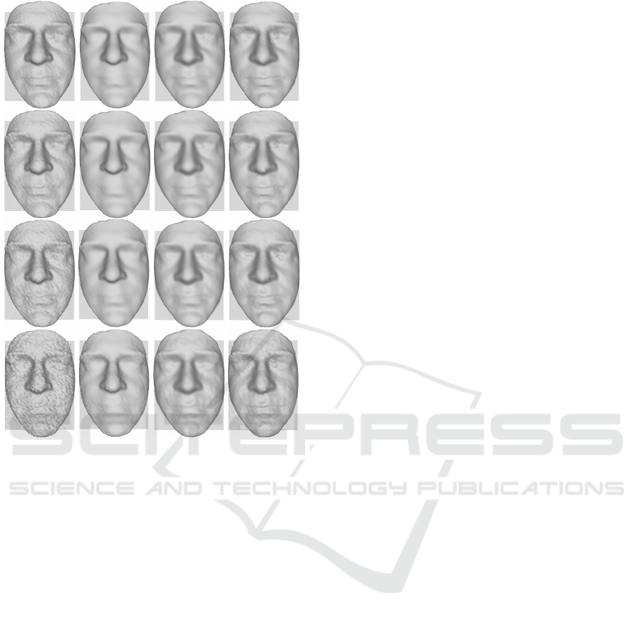
Figure 6: This ﬁgure shows the results obtained by the

tested ﬁlters. Each row shows the noise level applied to the

models which are 0.5, 0.7, 1.0, and 2.0 (respectively) mul-

tiplied by standard deviation. Column one illustrates the

noisy model, column 2, 3 and 4 show ﬁltered models by the

bilateral, gaussian ﬁlters, and ours respectively.

and depth translation.

As stated, the predictor performs a nearest neigh-

bor searching which implemented using a Kd-Tree to

accelerate it. In addition, we perform a dimensional-

ity reduction of the neighborhoods of each FFP re-

gion by using PCA (Hertzmann et al., 2001) of the

normalized neighbourhoods.

Our method has only a parameter to adjust, the

k size of the neighbourhood. This value depends on

the correlation length of the facial features on each

region. It is calculated, per each region, according

to the correlation length of all respective neighbour-

hoods (Pierce et al., 2000).

4.2 Correction

The ﬁltering process consists of modifying the ∆

points position according to the predictor. For each

point p ∈ ∆ (i), we determine its respective region

(FFP), (ii) get its neighborhood, normalize it (with

the respective mean and variance), to ﬁnally (iii) ap-

ply the projection in the base of the PCA. We use

the normalized and reduced neighborhood in the pre-

diction process. The predictor returns normalized Z-

value of the central point of the best matching neigh-

bourhood. Therefore, we take this value and multiply

it by the variance, and add it up to the average of p ∈ ∆

neighbourhood.

The normalization of the exemplar and target

neighborhood ensures that we can compare them ir-

respective of scale (division by variance) and transla-

tions in depth (subtraction by the mean). In addition,

it is noteworthy that a neighbourhood of the exem-

plar is normalized with its mean and variance, but the

process of unnormalization is performed by using the

mean and variance of the neighborhood of the target

that is being corrected. Thus, we transfer the neigh-

borhood feature of the exemplar to the target, with the

invariance mentioned above. Figure 4 illustrates this

step.

5 RESULTS AND CONCLUSIONS

The initials results were generated using a set of ex-

emplars based on the Bosphorus Database(Savran and

Sankur, 2017). It is intended to research on 3D and

2D human face processing tasks including expression

recognition, facial action unit detection, facial action

unit intensity estimation, face recognition under ad-

verse conditions, etc.

In order to evaluate the results, we performed the

experiments by applying a white noise (Boyat and

Joshi, 2015) to the set of different models. We varied

the noise intensity and compared the results with Bi-

lateral ﬁlter (Tomasi and Manduchi, 1998) and Gaus-

sian ﬁlter.

Afterwards, we calculated the mean-squared er-

ror (MSE) (Lehmann and Casella, 1998) between the

noisy models and ﬁltered models. Table 1 shows the

quantitative errors on the models used in this experi-

ment. Our method presents the minimum error com-

pared to the others ﬁlters, and preserves the details of

the mesh (sharpness). These sharp details can be seen

in Figure 6 (d).

Figure 5 shows the differences between the results

obtained by tested the methods. First column illus-

trates the applied noise, column 2, 3 and 4 show the

difference between the noisy model and the model ﬁl-

tered by the bilateral, gaussian ﬁlters and ours, respec-

tively. The noise is a random number in the interval

[−ασ, ασ], where σ is the standard deviation of the

target model. The alpha values per row are: 0, 0.5,

0.7, 1.0, 2.0 and 5.0.

Figure 6 exhibits the results obtained by the tested

A Content-aware Filtering for RGBD Faces

275

Table 1: This table shows the quantitative errors on the

models used in this experiment. The ﬁrst column is the

noise level. Column 2, 3 and 4 are the results of the mean-

squared error(MSE) (Lehmann and Casella, 1998) between

the noisy models and ﬁltered models.

Noise level Bilateral Gaussian Ours

Filter Filter

0.0 0.6615 1.8459 0.4859

0.5 0.6782 1.8484 0.4991

0.7 0.6970 1.8595 0.5289

1.0 0.7117 1.8819 0.5383

2.0 0.8236 1.9450 0.7218

5.0 2.1309 2.4487 2.1667

ﬁlters. Column one illustrates the noisy model (α

equals to 0.5, 0.7, 1.0 and 2.0), column 2, 3 and 4

show ﬁltered models by the bilateral, gaussian ﬁlters

and ours respectively.

Figure 7 illustrates the correction of a mesh ob-

tained using DephtSense camera (Sony, 2018). We

ﬁrst standardized the scale and sampling frequency

regards to the database, and then we corrected using

our ﬁlter.

(a) (b)

Figure 7: This Figure illustrates the correction of a mesh

obtained using DephtSense camera (Sony, 2018). We ﬁrst

standardized the scale and sampling frequency regards to

the database, and then we corrected using our ﬁlter. Figure

(a) shows the acquired noisy mesh, (b) is only the texture,

texture.

Figure 8: This Figure shows the results obtained by our ﬁl-

ter on different models. First column illustrates the model

with texture, column 2 shows the ground truth of the mesh

obtained by a 3D scanner, third column is the same mesh

after noise, fourth column shows ﬁltered models by our

method without texture and column 5 shows the textured

ﬁltered models.

Figure 8 demonstrates the results obtained by our

ﬁlter on different models. First column illustrates the

model with texture, second column shows the ground

truth of the mesh obtained by a 3D scanner, third col-

umn is the same mesh after noise, and fourth column

shows ﬁltered models by our method without texture.

The use of Bosphorus Database (Savran and

Sankur, 2017) allows us to use these models as a

ground truth. Currently, we are using 20 models as

exemplars randomly chosen. A future work may be

to determine the minimum amount of exemplar that

minimizes ﬁltering error. Reduction of the amount of

neighbourhoods per FFP region (by removing intra-

class redundancy) is left as future work.

Finally, our ﬁltering approach is based on a divi-

GRAPP 2019 - 14th International Conference on Computer Graphics Theory and Applications

276

sion of the model in regions in which all points have

an intrinsic geometric similarity. We presented how to

deﬁne these regions for the speciﬁc case of faces with

the usage of facial features. Regarding others kinds

of models, it is necessary to use a feature detector that

satisﬁes the three conditions presented in Section 4.1.

A future work direction is to deﬁne general descrip-

tors that can be used for general purpose ﬁltering.

REFERENCES

Aurenhammer, F. (1991). Voronoi diagrams—a sur-

vey of a fundamental geometric data structure. ACM

Comput. Surv., 23(3):345–405.

Botsch, M., Pauly, M., Kobbelt, L., Alliez, P., L

evy, B.,

Bischoff, S., and R

ossl, C. (2007). Geometric model-

ing based on polygonal meshes. In ACM SIGGRAPH

2007 Courses, SIGGRAPH ’07, New York, NY, USA.

ACM.

Boyat, A. K. and Joshi, B. K. (2015). A review paper: Noise

models in digital image processing. ArXiv e-prints.

Cho, H., Lee, H., Kang, H., and Lee, S. (2014). Bilateral

texture ﬁltering. ACM Trans. Graph., 33(4):128:1–

128:8.

de Berg, M., Cheong, O., van Kreveld, M., and Overmars,

M. (2008). Computational Geometry: Algorithms and

Applications. Springer.

Desbrun, M., Meyer, M., Schr

oder, P., and Barr, A. H.

(1999). Implicit fairing of irregular meshes using

diffusion and curvature ﬂow. pages 317–324, New

York, NY, USA. ACM Press/Addison-Wesley Pub-

lishing Co.

GmbH, R. (2018). Light ﬁeld technology.

Hertzmann, A., Jacobs, C. E., Oliver, N., Curless, B., and

Salesin, D. H. (2001). Image analogies. In SIG-

GRAPH.

Kazemi, V. and Sullivan, J. (2014). One millisecond face

alignment with an ensemble of regression trees. In

2014 IEEE Conference on Computer Vision and Pat-

tern Recognition, pages 1867–1874.

Lehmann, E. and Casella, G. (1998). Theory of Point Esti-

mation. Springer Verlag.

Liu, B., Cao, J., Wang, W., Ma, N., Li, B., Liu, L., and Liu,

X. (2018). Propagated mesh normal ﬁltering. Com-

puters & Graphics, 74:119 – 125.

Lu, X., Deng, Z., and Chen, W. (2016). A robust scheme

for feature-preserving mesh denoising. IEEE Trans-

actions on Visualization and Computer Graphics,

22(3):1181–1194.

Microsoft (2018). Kinect for windows.

Ng, R., Levoy, M., Br

edif, M., Duval, G., Horowitz, M.,

Hanrahan, P., et al. (2005). Light ﬁeld photography

with a hand-held plenoptic camera. Computer Science

Technical Report CSTR, 2(11):1–11.

Perona, P. and Malik, J. (1990). Scale-space and edge de-

tection using anisotropic diffusion. IEEE Transac-

tions on Pattern Analysis and Machine Intelligence,

12(7):629–639.

Pierce, L., Liang, P., Dobson, M. C., and Ulaby, F. (2000).

Texture correlation length: a deconvolution method to

account for speckle in sar images. In IGARSS 2000.,

volume 7, pages 2906–2908 vol.7.

Savran, A. and Sankur, B. (2017). Non-rigid registra-

tion based model-free 3d facial expression recogni-

tion. Comput. Vis. Image Underst., 162(C).

Sony (2018). Sony depthsensing solutions.

Stereolabs (2018). Zed 2k stereo camera.

Taubin, G. (1995). A signal processing approach to fair

surface design. SIGGRAPH ’95, pages 351–358.

Tomasi, C. and Manduchi, R. (1998). Bilateral ﬁlter-

ing for gray and color images. In Sixth Interna-

tional Conference on Computer Vision (IEEE Cat.

No.98CH36271), pages 839–846.

Wang, N., Gao, X., Tao, D., Yang, H., and Li, X. (2018). Fa-

cial feature point detection: A comprehensive survey.

Neurocomputing, 275:50 – 65.

Wei, L.-Y., Lefebvre, S., Kwatra, V., and Turk, G. (2009).

State of the art in example-based texture synthesis.

Eurographics STAR.

Wei, M., Huang, J., Xie, X., Liu, L., Wang, J., and Qin, J.

(2018). Mesh denoising guided by patch normal co-

ﬁltering via kernel low-rank recovery. IEEE Transac-

tions on Visualization and Computer Graphics, pages

1–1.

Yagou, H., Ohtake, Y., and Belyaev, A. (2002). Mesh

smoothing via mean and median ﬁltering applied to

face normals. In GMP, pages 124–131.

Zhang, Z. (1994). Iterative point matching for registration

of free-form curves and surfaces. Int. J. Comput. Vi-

sion, 13(2):119–152.

Zheng, Y., Fu, H., Au, O. K., and Tai, C. (2011). Bi-

lateral normal ﬁltering for mesh denoising. IEEE

Transactions on Visualization and Computer Graph-

ics, 17(10):1521–1530.

A Content-aware Filtering for RGBD Faces

277