Applications of Sparse Modelling and Principle Component Analysis

for the Virtual Metrology of Comprehensive Multi-dimensional

Quality

Sumika Arima

, Takuya Nagata

, Huizhen Bu

and Satsuki Shimada

Faculty of Engineering, Information, and Systems, University of Tsukuba, Tsukuba, Ibaraki Pref., Japan

Graduate School of Systems and Information Engineering, University of Tsukuba, Tsukuba, Ibaraki Pref., Japan

Keywords: Virtual Metrology (VM), PCA (Principal Component Analysis), LASSO (Least Absolute Shrinkage and

Selection Operator), Support Vector Machines (SVM), Multi-class Discrimination, Variable Extractions.

Abstract: This paper discussed the virtual metrology (VM) modelling of multi-class quality to describe the

relationship between the variables of a production machine's condition and the estimated/forecasted product

quality soon after finishing the machine processing. Applications of PCA and LASSO technique of the

Sparse modelling were introduced to define the multi-dimensional quality. Because the high accuracy and

quick computations are required for the VM modelling, in this study, the PCA-LASSO combination was

applied before building the VM models based on the kernel SVM (kSVM), particularly the linear kernel for

real-time use. As the result of evaluation of a CVD (Chemical vapor deposition) process in an actual

semiconductor factory, LASSO and linear-SVM could reduce the scale of the machine variable's set and

calculation time by almost 57% and 95% without deterioration of accuracy even without PCA. In addition,

as the PCA-LASSO, the multi-dimensional quality was rotated to the orthogonality space by PCA to

summarize the extracted variables responding to the primary independent hyperspace. As the result of the

PCA-LASSO combination, the scale of machine variables extracted was improved by 83%, besides the

accuracy of the linear-SVM is 98%. It is also effective as the pre-process of Partial Least Square (PLS).

1 INTRODUCTION

Semiconductor manufacturing is characterized by a

sequence of sophisticated manufacturing processes,

often exceeding several hundred production steps.

The process basically consists of main 10 or less

types of processes repeated, for example, washing,

deposition of materials on a semiconductor wafer, a

photo-lithography, an etching, a polishing, an

annealing, an intermediate test, and so on (Y.Naka,

K.Sugawa, and C. McGreavy, 2012).

Here the intermediate test is a quality check process

which occupies 30% of the whole of the production

process. Though the intermediate test aims the fast

detection of the quality defects to prevent to pile

more cost and time before the final test, the time and

the cost for the intermediate test is also serious in

100%-inspections ． Virtual metrology (VM) has

become widely studied all over the world to reduce

both the defects and the cost of the test (or the test

itself) as the research area of “advanced process

control” since 2005 as in AEC/APC (Advanced

equipment control/Advanced process control)

symposium around the world.

2 QUALITY DISCRIMINATION

MODELLING FOR VIRTUAL

METROLOGY

This study has advanced in 3 phases. As the first,

Arima (2011) applies kSVM for multi-class VM

modelling mainly for high accuracy. Second is the

application of the LASSO (Least Absolute

Shrinkage and Selection Operator) for automatic

variable extractions and fast computation of kSVM

(Arima, Ishizaki, and Bu, 2015). The third phase is

for all of those; automated variable extraction, the

high accurate quality detection, and the fast

computation. This paper mainly describe the third

phase in Section 3 after explaining the results and

354

Arima S., Nagata T., Bu H. and Shimada S.

Applications of Sparse Modelling and Principle Component Analysis for the Virtual Metrology of Comprehensive Multi-dimensional Quality.

DOI: 10.5220/0007385603540361

In Proceedings of the 8th International Conference on Operations Research and Enterprise Systems (ICORES 8th International Conference on Operations Research and Enterprise Systems),

pages 354-361

ISBN: 978-989-758-352-0

issues of the first and the second phases in this

section.

2.1 Problem Descriptions

The target process in this study is a plasma-CVD

(Chemical vapor deposition) process. CVD is one

type of thin-film formation processes and uses the

vapor process of a target material such that the snow

falls into the ground. The thickness of the film is

measured by nine points on a wafer after the CVD

process as the quality test for the CVD process

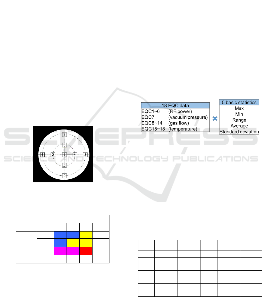
(Fig.2-1). Note that there are some types of layout of

the nine points. The measured data is composed into

2 factors (dimensions), “Design conformity (Dc)”

and “Uniformity (Uf)” for every wafer. Table. 2-1

shows one example of nine classes (3x3).

Not only Dc but also Uf is very important because

the larger wafer size leads the more defects besides

the higher throughput [wafers/unit time]. For

example, 30mm-size wafer is used in the target

factory, and the thickness sometimes much varies on

a wafer. The thickness influences the final quality of

the product such as the electrical resistance and the

current value.

Figure 2-1: Film thickness measured by nine points.

Table 2-1: Multi-dimensional quality class definition (nine

classes for 2-dimension).

For VM, quality was categorized by multi classes of

2 factors (dimensions), “Uniformity” and “Design

conformity” as shown in Table.2-1. Table 2-1

shows the case of nine classes as the result of 3-class

definition for each factor. The measures and

thresholds depend on the definition of the class. For

example of Table. 2-1, Dc was defined by the sum

total of square error between designed and actual

film thickness, and the boundaries of classes ‘A' and

‘B' or ‘B' and ‘C' were set as 3-quantiles between the

minimum and maximum values. Surface uniformity

(Uf) was defined by the standard deviation of the

film thickness, and the boundaries of classes ‘a' and

‘b' or ‘b' and ‘c' were set similarly as 3-quantiles.

This is only one example as the first phase

definition. The i-th wafer belongs to one of those

3x3=9 classes, and maintains the multi-dimensional

quality class expression as YC (i). Number in

Table.2-1 is the probability of the sample data. Note

that a different engineering action should be done

for the different colour in it.

On the other hand, conditions of a production

machine, used to explain the product quality, are

monitored on 18 sensors (EQC) settled in four types

of subunits of a machine (Fig.2-2). Soon after the

process end, 5 basic statistics are calculated, and 90

variables can be used for VM. Note that the original

wave data of each EQC cannot be opened for any

publications, and the statistics are used in this paper.

Figure 2-2: Machine variable set for experiment.

The challenge of VM here is to estimate/predict the

class of each product quality only by using the

machine data and the VM model that has been

learned by the set of machine data and the class data

of each product quality in a learning data set.

Table.2-2 shows the combinations of machine

variables to evaluate the VM accuracy. Note that

only the average and the standard deviation (SD) for

each EQC are used for the first phase. The choice of

the statistics is also based on engineering knowledge.

Table 2-2: 13 combinations of machine variables for the

performance evaluations ((x): # of variables).

a b c abc

46 18 6 70

14 2 8 24

2 0 4 6

ABC

62 20 18 100

Design

conformity

Uniformity

parameter

set No.

Avarage SD

parameter

set No.

Avarage SD

EQC1-18(18)

EQC1-18(18) 8 EQC8-14(7) EQC8-14(7)

EQC1-18(18)

- 9 EQC8-14(7) -

3 - EQC1-18(18) 10 - EQC8-14(7)

4 EQC1-6(6) EQC1-6(6) 11 EQC5-18(7) EQC5-18(7)

5 EQC1-6(6) - 12 EQC5-18(7) -

6 - EQC1-6(6) 13 - EQC5-18(7)

7 EQC7(1) EQC7(1)

Applications of Sparse Modelling and Principle Component Analysis for the Virtual Metrology of Comprehensive Multi-dimensional

Quality

355

2.2 The First Phase – SVM

Applications

As the first, S. Arima (2011) has examined VM of an

actual plasma-CVD process. Before applying the

kSVM, 2σ/3σ methods and the combination of the

Hotelling-T

and Q-statistics are evaluated for easier

2-class discrimination problem. The former is a

basic statistical process control (SPC), and the latter

is a representative of the multivariate statistical

process control (MSPC). The accuracy of the latter

stays low (67%) though a false error (False Positive

of confusion matrix) is much improved than the

former case. The reason why the low accuracy is

that the data is not ideally distributed along the

normal distribution, for example, subunit4:

temperatures.

Support Vector Machines (SVM) was originally

introduced to address the Vapnik’s (1995) structural

risk minimization principle and is now famous for

high accuracy in application fields (e.g. Lee,et.al.,

2015). The basic idea of SVM is to map the data into

a higher dimensional space called feature space and

to find the optimal hyperplane in the feature space

that maximizes the margin between classes as shown

in Fig.2-3. A kernel function, such as the

Polynomial, the Gaussian (hereafter RBF: Radial

basis function), the Linear, or the Sigmoid kernel are

used to map the original data to feature space. the

simplest SVM deals with a two-class classification

problem—in which the data is separated by a

hyperplane defined by a number of support vectors.

Support vectors are a subset of the training data used

to define the boundary between the two classes.

The kernel-SVM (kSVM) is compared with the

linear discriminant analysis for the binary

classifications problem as the first. The kSVM

performs better than the linear discriminant analysis

for the 2-class model, though each of those achieves

more than 80% of accuracy. Next is the multi-class

discriminant in Table.2-1. The linear and the

nonlinear discriminant analyses are compared with

the kSVM (Fig. 2-4). Here, SVMs were originally

designed for binary classifications. However, many

real-world problems have more than two classes.

Most researchers view multi-class SVMs as an

extension of the binary SVM classification problem

as summarized by Wong and Hsu (2006). Two

approaches, one-against-all and one-against-one

methods, are commonly used. The one-against-all

method separates each class from all others and

constructs a combined classifier. The one-against-

one method separates all classes pairwise and

constructs a combined classifier using voting shemes

In this study, the former approach is used.

Independent from the combination of machine

variables, the kernel-SVM achieves the best in the

three methods. Beside that, the accuracy of the

standard linear and non-linear discriminations (5-

dimension) are less than 60% and 20%, respectively.

100% accuracy is achieved when the variables of all

machine sub-units are used for the RBF-SVM

learning (x=1, 2, or 3).

However, it also shows that when there are not

enough variables in the data set for leaning step, the

accuracy in the test step stays lower level. Since the

semiconductor manufacturing is going to be a high-

mix and low-volume production system in these

years, and the number of samples can be used in the

learning step (is limited to several tens in some

cases. Therefore, we applied LOOCV (leave-one-out

cross-validation) to the problem. LOOCV involves

using one sample as the validation data in the test

step and the remaining samples as the training data

in the learning step. This is repeated on all samples

one by one to cut the original samples on a

validation data and the training data. We confirmed

the high accuracy of SVM using LOOCV to respond

to such a case of small data set. The 9-class

discrimination can be solved by using several tens

samples in this study. However, note that the

accuracy of kSVM model depends on the variables

considered, the number of classes, and the data size.

Figure 2-3: Kernel SVM: (a) non-linear discrimination

needed and (b) mapping from original space to feature

space by a kernel function.

As the summary of the first phase, SVM was applied

to construct an accurate VM model that provided

multi-class quality prediction of the product. The

VM model predicted with 100% accuracy the quality

of the product after a CVD process. The accuracy

depends on the set of input variables, and the best

here is a case variables of all subunits are included.

We got the following issues for the practical use in

the mass production as the result of the SVM

applications of the first phase:

1) Machine variables are selected manually based on

ICORES 8th International Conference on Operations Research and Enterprise Systems - 8th International Conference on Operations

Research and Enterprise Systems

356

Figure 2-4: Case#2 -VM accuracy -nine classes.

(x={1,2,…13}: # EQC variables set in Table 2-2 ).

the engineering knowledge, and the best

combination of the variables are empirically

detected. The issue is to automatically extract the

variables from the wider scope.

2) SVM using the RBF kernel could achieve the

highest accuracy for the VM model as the result of

comparison of the Polynomial kernel or the Sigmoid

kernel. However, for the large model it is difficult to

build the VM model based on RBF-SVM in a

realistic time period. For example, 10 hours for

learning when RBF is used for the final test process

of an actual factory. The issue is to utilize a different

kernel function of high speed without unallowable

deterioration of the accuracy.

2.3 LASSO Applications

Second phase is for automatic variable extractions

and fast computation of SVM learning, and so

LASSO technique is applied and evaluated.

2.3.1 Problem Definition

In the first phase, much adaptive accuracy of RBF-

SVM could be evaluated by numerical experiments

of discrimination of multi-class quality by using

actual fab data. However, 13 different variable sets

are comparably evaluated to get the best accuracy in

that case. The number of the variables (M=90) are

larger than the number of samples (e.g. n=50), and

thus some of those are selected based on engineering

knowledge (Table.2-2). Here, the sparse modelling

is a rapidly progressing in recent. It is one important

research area of the compressed sensing, and it has

very wide application fields such as a medical data

processing (rapid image sensing of MRI or CT), the

earth science (data-driven modelling and

forecasting), and so on. Note that the deep learning

method also can extract meaningful variables but it

requires a big data to analyze, and so it cannot be

used in this case. This paper focuses on the

automatic variable extraction which can be used even

when M >n.

2.3.2 Methods - Lasso

Basic Least-square method is used to estimate

coefficients C to minimize the estimation error

(Eq.2) in the linear regression (Eq.1) from the data

set { }. Here, if

some variables in x may not contribute to estimate

Y, some of values in “C” should be zero to reduce

the variance of the estimation result. That responds

to “parse” case. LASSO proposed by Tibshirani

(1996) is the estimation method of the sparse

coefficient vector to reduce the variance of the

estimation result (Eq.3).

















































(1)









 



















 





(2)







  

























(3)

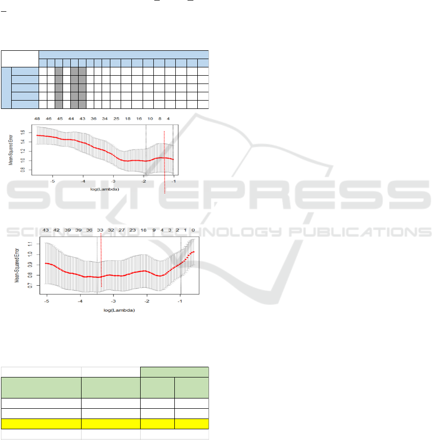
2.3.3 Numerical Results

In case of the class definition of Fig.2-1, we

empirically selected variables of 2 kinds of statistics

as the result (Table.2-2). Here, we try to

“automatically extract the variables by applying the

sparse modelling, and evaluate those accuracy as

well. The significant variables for the design

conformity (V(D)) and for the uniformity” (V(U))

are extracted (Table.2-4). The-10-hold cross

validation is used for LASSO, and the set of

variables are selected when the lambda is minimum

as shown in Figures 2-5 and 2-6.

VM model of kSVM is built by using conjoint

form of variables (e.g. V(D)V(U)) as the first case.

Its accuracy of each kernel is evaluated for 2-

demensional quality classification by using the

LOOCV. A linear kernel is the best for the Lasso-

kSVM as shown in Table 2-5.

2.3.4 Issues for the next

We got the following issues for the practical use in

the mass production as the result of the SVM

applications of the second phase. Automated

procedure of VM modelling should be proposed.

1) LASSO regression model can achieve the

compression of the variables and computational time

Applications of Sparse Modelling and Principle Component Analysis for the Virtual Metrology of Comprehensive Multi-dimensional

Quality

357

much, however, we have to consider about the

multi-objective model. The multi-dimensional

classes of product quality may not be in the

relationship of linearly independent each other

because it has been defined by the engineering

knowledge. In that case, the join set of variables can

be redundant. The exclusion is still 7 variables as

common of Dc and Uf (Table 2-4).

2) It is required to compare with other multi-

objectives models such as PLS (Partial Least

Squares) often used in chemo-metrics research area.

Table 2-4: Variable extractions by Lasso -(Design

conformity(D) / Uniformity (U) /Both (B)).

Figure 2-5: Cross validation for Lasso parameter (λ -

[min, lse] = [ 0.1462973, 0.3540583] ) for i) D.

Figure 2-6: Cross validation for Lasso parameter ( λ -

[min, lse] = [0.03037, 0.37440] ) for ii) U.

Table 2-5: VM accuracy – Lasso-kSVM.

3 PCA AND LASSO

APPLICATIONS

3.1 Problem Definition

In this section, we will discuss an automated VM

procedure using PCA-LASSO and the kernel SVM

to solve the issues mentioned in section 2.3.4. PLS is

able to analyze the case the sample size is less than

the number of the variables.

3.2 Method - PCA and PLS

3.2.1 Basics of PCA and PLS

Principal component analysis (PCA) is a

mathematical procedure that transforms a number of

possibly correlated variables into a smaller number

of uncorrelated variables called principal

components. PCA rotates the axes of the original

variable coordinate system to new orthogonal axes,

called principal axes, such that the new axes

coincide with directions of maximum variation of

the original observations (Fig.3-1(graph)).The

regression is the modelling of relational expression

between the objective variable(s) Y and the

explanatory variables X. Coefficients are estimated

under the conditions of lowest estimation errors by

the Least-square or another method. There are some

regression models using PCA (Fig.3-1). PCR is a

representative in which PCA is applied only to X.

On the other hand, both X and Y are rotated by PCA

before regression in PLS.

3.2.2 PCA Application for Quality

Definitions

The PCA is applied for a multi-dimensional quality

definition. As the first case, PCA is used to 2-

demensional quality data (Design conformity (Dc)

and Uniformity (Uf)) to rotate to the orthogonality

space. After the PCA, the class is defined under the

threshold of 3-quantiles for each dimension. In the

second PCA application, we newly define the multi-

dimension of the quality as shown in Table.3-2 as

the result of PCA using original thickness values of

9 points. The primary principle component (PC1)

shows the level of thickness and it responds to the

“Design conformity” (Dc’). The second and the third

principle component (PC2, PC3) show the deflection

of the thickness and respond to “Uniformity” (Uf ’).

The threshold of quality class can be defined by:

i) Probability (e.g. normal distribution case)

1 2 3 4 5 6 7 8 9 10 11 12 13 14 15 16 17 18

Min U U U U U U

Max U D U D U U B U B

Range U D U U U

Average B U U B B U D U U U

Std. dev. U U B U B U U

※D:Design conformity, U: Uniformity, B:Both

Sensor No.

statistics

Variables

extracted

Quality class of VM

variables set

[# of variables]

RBF Linear

Design conformity (A,B,C) V(D) [11] 92 88

Uniformity (a,b,c) V(U) [35] 84 100

2D quality (A,B,C) X (a,b,c)

V(D)∪V(U) [39] 90 100

accuracy [%]

Kernel

↑# of variables selected.

ICORES 8th International Conference on Operations Research and Enterprise Systems - 8th International Conference on Operations

Research and Enterprise Systems

358

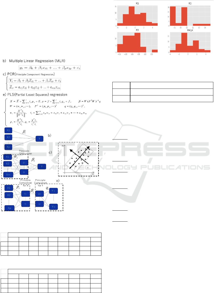
ii) Quantiles (e.g. uniform distribution case, etc.)

Based on the distribution of the principal component

scores (Fig. 3-3), only PC1’s score is statistically

adapt to the normal distribution as the result of One-

sample Kolmogorov-Smirnov test (D = 0.55944, p-

value = 2.998e-15, alternative hypothesis: two-

sided). Here, i) is selected for defining classes of Dc’

and ii) is used for defining classes of Uf ’. The

threshold here is defined as shown in Table 3-5 for i).

On the other hand, the 3-quantiles is used for ii).

Figure 3-1: Multivariate regression models.

Table 3-1: PCA result - factor loading (PC1, 2, 3).

Table 3-2: PCA result - factor loading (PC1, 2, 3).

Figure 3-3: PCA result -principal component scores.

Table 3-5: The threshold for i (yi: the score,

standard deviation).

3.3 Numerical Results

3.3.1 Automated VM Procedure

The procedure of PCA-LASSO and kSVM

STEP-1: PCA to define the multi-dimensional

quality. Select a few principal components by the

cumulative contribution ratio becomes over 80*% or

so. (*depend on the target accuracy)

STEP-2: LASSO to extract the significant machine

variables

STEP-3: Select the principal component to use in the

following step. Check the LASSO result (e.g. PC2

is excepted because of no variables selected.)

STEP-4: Select the threshold type for each PCs.

Check the distributions of principal component

scores for selected PCs (e.g. PC1 and PC3 is set to

the probability-type and to the quantiles)

STEP-5: Define the class for all samples (e.g.

product wafer here)

STEP-6: SVM learning and class discriminations.

3.3.2 PCA-LASSO (1) and Kernel SVM

As the first case, PCA is used to 2-demensional

quality data (Dc2 and Uf2) to rotate to the

orthogonality space. The threshold of quality class

can be defined by the 3-quantiles for each dimension.

Combination of LASSO and linear-SVM appear the

best accuracy again (100%) even if PCA is used. In

the same case, the accuracies of RBF-SVM and

Polynomial-SVM result 82% and 92%, respectively.

In case of PCA-LASSO (1), PC2 is excepted

because no machine variables are selected in the

LASSO regression, and only the primary principle

QC1 QC2 QC3 QC4 QC5 QC6 QC7 QC8 QC9

PC1 0.292 0.350 0.350 0.335 0.352 0.350 0.303 0.288 0.370

PC2 0.177 0.189 0.263 0.454 0.076 0.010 (0.333) (0.076) (0.731)

PC3 (0.660) 0.087 0.126 0.390 0.155 (0.030) (0.396) (0.260) 0.373

Original variables of quality measured

QC1 QC2 QC3 QC4 QC5 QC6 QC7 QC8 QC9 Average

PC1 0.292 0.350 0.350 0.335 0.352 0.350 0.303 0.288 0.370 0.332

PC2 0.177 0.189 0.263 0.454 0.076 0.010 (0.333) (0.076) (0.731) 0.003

PC3 (0.660) 0.087 0.126 0.390 0.155 (0.030) (0.396) (0.260) 0.373 (0.024)

original variables of quality

Principal

components

(PCA )

a 　μ-σ≦yi≦μ+σ

b μ-2σ≦yi<μ-σ, μ+σ<yi≦μ+2σ

c yi<μ-2σ, μ+2σ<yi

PC1

PC2

Applications of Sparse Modelling and Principle Component Analysis for the Virtual Metrology of Comprehensive Multi-dimensional

Quality

359

component (PC1) represents both the “Design

conformity” and “Uniformity” (PC1: Dc2 & Uf2).

Note that PLS regression cannot work well in this

case. Error is detected in calculation.

3.3.3 PCA-LASSO (2) and Kernel SVM

Here we use the result of PCA using original

thickness values of 9 points (PC1: Revised design

conformity (Dc’), PC3: Revised uniformity (Uf ’)).

-principal component PC2 is excepted because no

machine variables are selected by LASSO.

Three principal components were obtained by PCA,

and 12 variables for PC1 and 4 variables for PC3

were chosen. Variable sets for PC1 and PC3 are

expressed as and 







 Since each principal

component is orthogonal, the variables chosen for

each principal component tend to be uncorrelated,

that is, they are exclusive. Thus, variables included

in the union can explain the original objective

variables without waste. The variable set used for

the SVM learning is defined as the union of the

variables extracted by LASSO:   

Linear-SVM appears again the best accuracy for all

(98%) in addition to the shortest computational time.

RBF-SVM is lower accuracy (82%) though it can

keep its accuracy based on best parameters for the

gamma function. In addition, the computational time

is the largest for all. The accuracy of the

Polynomial-SVM stays about 90%.

Note that the result of the variable extraction of this

PCA-LASSO is helpful pre-process for PLS

regression though the PLS regression cannot be

solved when the original input data without the

representative object variables and extracted

explanatory variables. This is one type of cases that

PLS regression does not go well because the data set

includes an explanatory (independent) variable

irrelevant to an objective (dependent) variable. Even

though in such a case, PLS regression can succeed

by the pre-process of variable extraction of the PCA-

LASSO regression. The best number of objective

variables, that is principal components here, is the

same as the number of selected objective variables

in PCA. “3” is the best of the lowest RMSE (root-

mean-square error) as shown in Fig. 3-4.

3.3.4 PCA-LASSO (3) and Kernel SVM

We can use the result of PCA to define

comprehensive index by using the contribution rate

(thus Eigen values), Eigen vectors, and so on.

However the result of LASSO for the

comprehensive index is not so effective here.

Figure 3-4: Selection of # of objective variables (principal

components here) for PLS.

3.4 Summary of Variable Extractions

PCA is combined to LASSO regressions instead of

PCR (Fig.3-1) or PLS (Fig.3-1, or as a pre-process

of PLS) to extract the optimal and smallest set of

variables for comprehensive VM modelling of

multi-dimensional quality. As the result of

comparison of PCA-LASSO (1) and (2), the

compaction rate is improved by about 66.7% and

83.3% besides the exclusion rate’ improvement

(Table 3-7). In case of PCA-LASSO (1), PC2 is

excepted because no machine variables are selected

in LASSO regression, and only the primary principle

component (PC1) represents both the design

conformity and uniformity (Dc2 & Uf 2:PC1). That

is caused the original definition of the 2 factors of

thickness is not linearly independent. In such a case,

compression rate is lower than the other case. The

exclusion rate becomes much lower in the proposed

PCA-LASSO cases (Tables 3-6, 3-8, 3-9, 3-10). See

appendix-A for the coefficients of the variables.

3.5 Conclusions of the Third Phase

In this section, automated VM procedure using

PCA-LASSO and kernel SVM is proposed and

evaluated. PCA is combined to LASSO regressions

instead of using PCR or PLS to extract the

reasonable and smallest set of variables for

comprehensive VM modelling of multi-dimensional

quality. In addition, the liner-kernel SVM using the

variables selected LASSO regressions achieves the

highest accuracy. LASSO and linear-kernel SVM

can compress the scale and computational time

much in the model learning without deterioration of

the accuracy.

ICORES 8th International Conference on Operations Research and Enterprise Systems - 8th International Conference on Operations

Research and Enterprise Systems

360

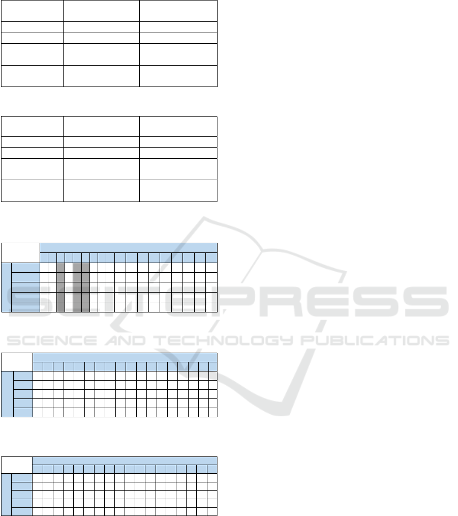
Table 3-6: The number of machine variables extracted.

Table 3-7: Compaction rate and Exclusion rate.

Table 3-8: Machine variables extracted by LASSO. (※

D: Design conformity, U: Uniformity, B:both).

Table 3-9: Variables extraction of PCA-LASSO (1). (※

PC1: Design conformity & Uniformity).

Table 3-10: Variables extraction of PCA-LASSO (2).

(PC1: Design conformity, PC3: Uniformity, B:both).

4 CONCLUSIONS

This study discussed the modelling of virtual

metrology in 3 phases. The first is the application of

SVM for multi-class virtual metrology mainly for

high accuracy. The second phase is LASSO

application for automatic variable extractions and

fast computation of Linear-SVM learning. Finally

the third phase is for all; automated extractions of

the best set of machine variables, the high accurate

quality discriminations for the multi-dimensional

classes, and the fast computation for a practical use.

ACKNOWLEDGEMENTS

We deeply appreciate the referees' advice and

comments. Also we thank ICORES secretariat for

their gentle guides.

REFERENCES

Y.Naka, K.Sugawa, C. McGreavy., 2012. Introduction to

VLSI Process Engineering, Springer.

APC Conference (USA) (Oct. 22

, 2018 access)

http://www.cvent.com/events/apc-conference-xxx-

2018/event-summary-

a8d0f8ae27e84ecf97862bdc1b4c7b01.aspx.

EUROPEAN ADVANCED PROCESS CONTROL AND

MANUFACTURING CONFERENCE (Oct. 22

2018 access): https://www.apcm-europe.eu/home/.

AEC/APC symposium Asia (Oct. 22

, 2018 access):

https://www.semiconportal.com/AECAPC/index_e.ht

ml.

Literatures in “Metrology” and “Advanced process control”

sessions of IEEE Transaction on Semiconductor

Manufacturing (since 2011).

S. Arima, 2011. Virtual Metrology-based Engineering

Chain Management by Multi-classification of Quality

using Support Vector Machine for Semiconductor

Manufacturing, Int. J. Industrial and Systems

Engineering No.8 Vol.1, Inderscience pub., pp.1-18 .

S. Arima., et.al., 2015. Applications of machine learning

and data mining methods for advanced equipment

control and process control, Proceedings of AEC/APC

symposium Asia 2015, DA-O-34 (pp.1-6).

Vapnik, V.N. ,1995. The Nature of Statistical Learning

Theory, New York: Springer-Verlag.

Wong, W. and Hsu, S. ,2006. Application of SVM and

ANN for image retrieval, European Journal of

Operations Research, Vol. 173, pp.938–950.

T. Lee, C. O. Kim., 2015. Statistical Comparison of Fault

Detection Models for Semiconductor Manufacturing

Processes, IEEE Trans. on Semi. Manufacturing,

28(1), pp.80-91, IEEE.

R.Tibshirani.,1996. Regression shrinkage and selection via

the lasso, J. R. Statist. Soc. B, 58(1), pp.267-288.

R. A. Johnson, D. W. Wichern., 2007. Applied

Multivariate Statistical Analysis, Prentice Hall.

# of variables (total)

V(D+U)=V(D)⋃V(U)

# of depricated variables

V(D*U)=V(D)∩V(U)

Original 90 -

LASSO (Dc, Uf)　 39 7

PCA-LASSO(1)

(pc1: Dc2 & Uf2)

30 0

PCA-LASSO(2)

(pc1: Dc', pc3:Uf')

15 1

[%]

Compaction rate

=(90-V(D+U))/90

Exclusion rate

={V(D+U)-V(D*U)}/V(D+U)

Original 0.00% -

LASSO (Dc, Uf)　 56.67% 82.05%

PCA-LASSO(1)

(pc1: Dc2 & Uf2)

66.67% 100.00%

PCA-LASSO(2)

(pc1: Dc', pc3:Uf')

83.33% 93.33%

1 2 3 4 5 6 7 8 9 10 11 12 13 14 15 16 17 18

Min U U U U U U

Max U D U D U U B U B

Range U D U U U

Average B U U B B U D U U U

Std. dev. U U B U B U U

Sensor No.

statistics

Variables

extracted

1 2 3 4 5 6 7 8 9 10 11 12 13 14 15 16 17 18

Min PC1 PC1 PC1 PC1

Max PC1 PC1 PC1 PC1 PC1 PC1 PC1 PC1 PC1

Range PC1 PC1 PC1 PC1

Average PC1 PC1 PC1 PC1 PC1 PC1

Std. dev. PC1 PC1 PC1 PC1 PC1 PC1 PC1

Sensor No.

statistics

Variables

extracted

1 2 3 4 5 6 7 8 9 10 11 12 13 14 15 16 17 18

Min PC1 PC3 PC1

Max PC1 PC1 PC1 PC1

Range PC1

Average PC3 PC1 B

Std. dev. PC3 PC1 PC1 PC1

Variables

extracted

Sensor No.

statistics

Applications of Sparse Modelling and Principle Component Analysis for the Virtual Metrology of Comprehensive Multi-dimensional

Quality

361