
Reaction-diffusion Woodcuts
D. P. Mesquita and M. Walter
Universidade Federal do Rio Grande do Sul, Porto Alegre, Brazil
Keywords:
Reaction-diffusion, Woodcuts, Expressive Rendering.
Abstract:
Woodcuts are a traditional form of engraving, where paint is rolled over the surface of a carved wood block
which will be used as a printing surface over a sheet of paper, so only the non-carved parts will be printed
in the paper. In this paper, we present an approach for computer simulated woodcuts using reaction-diffusion
as the underlying mechanism. First, we preprocess the segmented input image to generate a parameter map,
containing values for each pixel of the image. This parameter map will be used as an input to control the
reaction-diffusion processing, allowing different areas of the image to have distinct appearances, such as spots
or stripes with varied size or direction, or areas with plain black or white color. Reaction-diffusion is then
performed resulting in the raw appearance of the final image. After reaction-diffusion, we apply a thresholding
filter to generate the final woodcut black and white appearance. Our results show that the final images look
qualitatively similar to some styles of woodcuts, and add yet another possibility of computer generated artistic
expression.
1 INTRODUCTION
Non-photorealistic rendering (NPR) (Strothotte and
Schlechtweg, 2002), also known as Expressive Ren-
dering, always looked for inspiration in the many
forms of traditional artistic expression, trying to simu-
late the visual results of manual techniques. Since the
early work of Haeberli (Haeberli, 1990) this area of
research has seen major advances, being able to con-
vincingly simulate natural media effects such as pen-
cil drawing (Lu et al., 2012), oil painting in real-time
and on mobile devices (Stuyck et al., 2017), watercol-
ors (DiVerdi et al., 2013) (Wang et al., 2014), among
many others. Hegde, Gatzidis, and Tian present a re-
view of these artistic inspired results in (Hegde et al.,
2013). Among the many relief printing and artistic
techniques, such as etching or engraving, woodcuts
have a distinct look due to their nature. A block of
wood is used as the substrate where the artist draws
the scene by carefully carving the wood with spe-
cialized tools. A thin layer of usually black paint
is rolled over the wood substrate. The image is
formed by evenly pressing a white paper over the
wood block. The result is a black-and-white image
where the woodgrain is visible and contributes to the
appeal of the result.
In this paper, we present an approach to synthe-
size virtual woodcuts from natural images. We pro-
pose the use of reaction-diffusion (RD) systems as the
underlying mechanism to achieve the “feel and look”
of woodcuts. Our main contribution is the introduc-
tion of RD addressing an artistic technique not yet ex-
plored, with visually pleasing results.
2 RELATED WORK
There has been countless approaches to render 2D in-
put into artistic oriented renderings. The survey by
Kyprianidis and colleagues (Kyprianidis et al., 2013)
presents a taxonomy of Image-Based Artistic Render-
ings, as they name this class of techniques. Their fo-
cus was on the underlying methods and techniques be-
ing used rather than the artistic effect being simulated.
The chapter by Lai and Rosin (Lai and Rosin, 2013)
presents yet another survey with focus only on tech-
niques working with reduced color palettes, typical of
some artistic expressions such as comics, paper-cuts,
and woodcuts.
Virtual woodcuts have not attracted much atten-
tion from graphics researchers. Perhaps because it is
a less popular artistic technique than oil and water-
color paintings, for instance. Mizuno and colleagues
(Mizuno et al., 2006) implemented a virtual analog
of real woodcuts. With the use of a pressure sensi-
tive pen and a tablet, their system allowed the user the
feeling of carving real wood which could then be vir-
tually printed. Their work is perhaps the first to bring
Mesquita, D. and Walter, M.
Reaction-diffusion Woodcuts.
DOI: 10.5220/0007385900890099
In Proceedings of the 14th International Joint Conference on Computer Vision, Imaging and Computer Graphics Theory and Applications (VISIGRAPP 2019), pages 89-99
ISBN: 978-989-758-354-4
Copyright
c
2019 by SCITEPRESS – Science and Technology Publications, Lda. All rights reserved
89
the attention to woodcuts in the NPR field. Their vi-
sual results, however, did not look very convincing,
perhaps due to the need of artistic abilities to render
a scene. A year later, Mello, Jung and Walter (Mello
et al., 2007) introduced the first approach to synthe-
size woodcuts from natural images. Their approach
applied a sequence of image processing operations to
turn any image into a woodcut. Their results showed
some similarity with real woodcuts. In 2011 Win-
nemoller presented an extension on the Difference-
of-Gaussians operator allowing new results for artis-
tic renderings from images (Winnem
¨
oller, 2011). Al-
though his work did not particularly address wood-
cuts, he present one result mentioned as similar to
woodcuts.
Just recently we have seen new approaches to vir-
tual woodcuts. In 2015 a short paper (Li and Xu,
2015) addressed a particular style of color woodcuts,
known as Yunnan woodcuts. These are color wood-
cuts that use only a single wood block that is recarved
for each color. A year later the same researchers (Li
and Xu, 2016) extended their previous work, paying
particular attention to the color mixing intrinsic to the
technique.
RD was introduced by Turing (Turing, 1952) as a
mechanism to explain biological patterns. Basically,
two chemicals react until they reach a stable state.
Mapping their concentrations to colors we can see
patterns of stripes, spots, and labyrinthine ones. Al-
though it has been used in many graphics tasks before
(Turk, 1991) (Kider Jr. et al., 2011) (Barros and Wal-
ter, 2017), just recently RD has been explored in NPR
approaches. Chi and colleagues (Chi et al., 2016) ex-
plored these patterns for image stylization, achieving
many visually interesting results. A year later, Jho
and Lee (Jho and Lee, 2017) used the RD patterns in
a new method of tonal depiction. Both did not ad-
dressed woodcuts.
In this paper, we introduce a new method for syn-
thesizing virtual woodcuts from natural images adapt-
ing a RD system to the needs of rendering woodcut-
like results. Our visual results compare favorably both
with previous work and with commercial image ma-
nipulation software.
3 METHODOLOGY
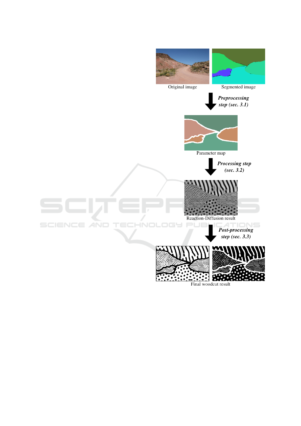
Our method is subdivided into three steps: prepro-
cessing, processing (RD) and post-processing (Fig.
1), as will be described below.
Briefly speaking, the preprocessing step receives
as input an image and returns a parameter map, where
each pixel receives a specific value for several param-
Figure 1: Pipeline of our methodology. First, we submit
an image and its segmentation to the preprocessing step, in
order to generate a parameter map. This parameter map is
then used as basis for the RD process, generating then a
raw woodcut-like image. Last, the RD result is filtered in
a post-processing step in order to improve its appearance,
generating the final woodcut image.
eters used in the processing step. The processing step
runs the RD mechanism over the parameter map, set-
ting the overall appearance of the final rendering. Fi-
nally, the post-processing step filters the RD result in
order to enhance the similarity with a real woodcut
image. We describe these steps below.
GRAPP 2019 - 14th International Conference on Computer Graphics Theory and Applications
90

3.1 Preprocessing
Our algorithm receives as input both an image to be
used as the basis for our final woodcut, and a seg-
mentation of this image. The input image is con-
verted to gray scale for all calculations used in our
work. Instead of computing a segmentation, we used
the dataset from ADE20k (Zhou et al., 2017). This
dataset contains 22,210 images, from landscapes to
indoor scenes, being visually adequate for our pur-
poses. Besides, each image has a semantic segmen-
tation. The segmented input image will be defined as
a collection of regions. In Table 1 we present the pa-
rameters used in the preprocessing step, which will be
explained throughout the text.
Table 1: User-defined parameters for the preprocessing
step. Details about each parameter are given in the text.
Parameter Default Value
n
dilate
1
T
low
25
T
high
210
T
size
500 pixels
k {1, 5, 9, 13, 17}
S
min
0.005
S
max
0.015
T
di f f
5.0
S
θ
0.010
The first step is to discriminate the parts of the
image where no RD pattern will be generated, and
instead a plain black or white color will be applied.
First, from observation of real woodcuts, we define
the borders of the segmented regions as black. These
borders define the scene and so they should appear in
the final woodcut as black strokes. The borders can
be thickened to the desired size by a dilate operation,
where, for every pixel in a binarized version of the
image (where borders are black and other pixels are
white), a kernel with dimensions 5 × 5 is used: if any
pixel inside this kernel is black, then the pixel in ques-
tion is marked as black; otherwise it is white. This
operation can be repeated n
dilate
times. Larger kernels
and/or larger values of n
dilate
result in thicker borders,
with smaller regions being absorbed into them.
According to (Mello et al., 2007), in real wood-
cuts the brightest regions are white, while the darkest
ones are black, in both cases without any discernible
stroke pattern. To reproduce this appearance, we use
the same mechanism of their work, where two thresh-
olds, T
low
and T
high
, are used; then we mark as white
and black any regions whose average gray-scale color
intensity is, respectively, higher than T
high
and lower
than T
low
. Finally, to reduce unnecessary noise, we
merge the smallest regions, whose area (i.e., the num-
ber of pixels) is smaller than a given threshold, T
size
,
into the borders, by marking these regions as black.
Fig. 2c shows an example of the black and white gen-
erated from this part of the preprocessing step.
To allow a variation of detail levels for different
parts of the image, we compute, for each pixel, a
value for a RD parameter related to the size of struc-
tures generated by this mechanism called S (Bard and
Lauder, 1974). We adapted the method from Hertz-
mann (Hertzmann, 1998) for this task. In that work,
different detail levels in a painting are simulated by
using distinct brush sizes in sequential steps, such that
regions where fine detail is needed are painted with
smaller brushes than other parts of the image, draw-
ing more attention toward these regions. In our work,
more detailed areas receive a higher value of S, result-
ing in smaller structures and thus increased preserva-
tion of details.
To implement this feature, we defined the follow-
ing parameters: a list of integers k, the maximum S
max
and minimum S
min
values of S, and an error thresh-
old T
di f f
. First, we mark all pixels as S
max
. Then,
for each integer k
i
, starting from the smallest one, we
generate a reference image by performing a Gaussian
blur using a k
i
× k
i
kernel (noting that larger values
for k
i
result in more blurred images, and so more dif-
ferent than the original). For every pixel, we com-
pute the average pixel-to-pixel difference between the
reference image and the original one for the entire
neighborhood of this pixel, in a window with the same
dimensions as the blur kernel. If this area differ-
ence is smaller than T
di f f
, we consider that the area
around this pixel did not change too much between
the blurred image and the original one, being conse-
quently less detailed. We mark this pixel as the value
of S corresponding to this kernel, calculated as:
S
i
= S
max
+ m ∗ (k
i
− min k)
m =
S
max
− S
min
mink − max k
Figure 2: Lighthouse image used in our tests. (a) Original
image from (Mello et al., 2007). (b) Manual segmentation
of this image. (c) Borders and areas without RD, calcu-
lated in the preprocessing step, already painted as white and
black. Areas where RD will occur are marked as gray.
Reaction-diffusion Woodcuts
91

After computing S for every pixel, we set a unique
S for each region by computing the average S inside
that region. By doing that, we ensure that inside a
region all strokes will have the same size, improving
structure size coherence for the result.
The parameter T
di f f
affects the average level of
detail and size of strokes: smaller values for T
di f f
re-
duce the chance of every step to set a smaller value
for S in the comparison between the original image
and the blurred one, resulting on larger values for S
and consequently smaller strokes, and a more detailed
final result.
After that, we need to calculate the orientation of
strokes. In our work, we have three options: a) orien-
tation by region, b) orientation by pixel, and c) adap-
tive orientation. In the orientation by region, every
pixel inside a given region will have the same orien-
tation, so strokes will be parallel to each other inside
the same region. As (Mello et al., 2007) observed, the
wood carvings tend to initiate in the brighter parts of
a region, so for every region we will start the strokes
from the brighter point near region borders. Firstly,
for each pixel of a given region which has at least one
border pixel as neighbor, we test the average lumi-
nance for a 5 × 5 window. We retrieve the pixel with
the highest average luminance inside its correspond-
ing window. Then, we compute the center pixel of
every region as the average of the horizontal and ver-
tical positions of every pixel in that region. To find the
orientation angle of a region we compute the slope of
the line formed by these two pixels: the border pixel
with the largest average luminance in its surroundings
and the central pixel, as follows:
θ
reg
= arctan
d
y
− c
y
d
x
− c
x
where θ
reg
is the orientation of strokes for a given re-
gion, d is the boundary pixel and c is the central pixel
of a given region.
When calculating orientation by pixel, it is possi-
ble to set different pixel-specific values for θ, which
allows the contour of small details to appear in the
resulting image. Our method for such calculation is
based on local orientation of luminance as used by
(Mello et al., 2007) and (Li and Xu, 2016). First, for
each pixel (i, j) in the image, we compute the local
average orientation of luminance Θ in a 5×5 window
W centered in that pixel as follows:
Θ
i, j
=
1
2
tan
−1
V
x
(i, j)
V
y
(i, j)
where
V
x
(i, j) =
∑
(u,v)∈W
2G
x
(u,v)G
y
(u,v)
V
y
(i, j) =
∑
(u,v)∈W
(G
x
(u,v)
2
− G
y
(u,v)
2
)
and G
x
and G
y
are the image gradients in the x and y
directions, calculated using the Sobel operator.
To orient the strokes preserving the contour de-
tails of the original image, their orientation should be
perpendicular to the local average orientation of lumi-
nance Θ. This happens because Θ follows the direc-
tion of color gradients, i.e., it goes from black areas
to white areas or vice-versa, being thus perpendicular
to any existing line in the image (since the lines have
more or less the same color). So, the stroke orienta-
tion θ for a pixel is given by the following formula:
θ
i, j
=
π
2
+ Θ
i, j
While more complex objects as an human body
or decorated buildings would need a finer level of de-
tail, in background areas as the sky a single orienta-
tion works better, so the user would focus on the fore-
ground instead of the background. The adaptive ori-
entation method allows us to use both methods, orien-
tation by region or by pixel, for different areas of the
image, depending on the detail level required by that
region. This detail level was encoded by the value of
S calculated for that region previously. For a given re-
gion with a S value equals to S
region
, if S
region
> S
θ
(an
user-defined threshold), then that region will use ori-
entation by pixel; otherwise, the region will use ori-
entation by region. Thus, regions with higher values
for S, and consequently more details in the original
image, will have these details preserved in the final
woodcut, using a pixel-specific orientation. Less de-
tailed regions will have a single orientation, enhanc-
ing their status as background regions.
Many real woodcuts show, besides lines and flat
color areas, dots or other similar structures. In our
RD system, it is possible to control which regions will
have stripes or spots. We simulate this pattern diver-
sity by setting different values of a parameter called δ
for every region. We considered brighter areas to have
spots and darker ones to have stripes, using the aver-
age color of each region to compute this parameter.
We will describe in the next section how this parame-
ter works, when we will detail the main engine of our
system, the RD process.
At the end of the preprocessing step, we save an
image with the same dimensions of the original to
be used as input for the RD process, where different
color channels are used to set the local value of dif-
ferent parameters calculated in this step as follows:
red for S, green for δ, and blue for the orientation an-
gle θ
reg
. Also, the value corresponding to plain white
(255 for all channels) is interpreted as absence of RD
for that pixel.
GRAPP 2019 - 14th International Conference on Computer Graphics Theory and Applications
92
Alternatively, it is possible to use an image with-
out segmentation, for cases where a segmentation is
not available. In this case, there will be no borders
or regions without RD, θ will necessarily be defined
by pixel and not by region, and each pixel will have a
different value for S, since there will be no region to
compute the average value for this parameter.
3.2 Processing
To generate the pattern of strokes, we use a RD sys-
tem, specifically the non-linear system defined by
(Turing, 1952) and later used by (Bard, 1981) (Bard
and Lauder, 1974). In Table 2 we present the param-
eters defined in the processing step. This system is
expressed by the set of partial differential equations
below:
∂a
∂t
= S(16.0 − ab) + D
a
∇
2
a
∂b
∂t
= S(ab − b − β) + D
b
∇
2
b
Here, a and b represent the concentration of mor-
phogens (the substances responsible for generate pat-
terns in Turing’s theory), ∂a/∂t and ∂b/∂t the respec-
tive rates of variation in time, ∇
2
a and ∇
2
b the Lapla-
cian representing the spatial variation of the mor-
phogens (so they can diffuse from areas of higher con-
centration to areas of lower concentration). D
a
and D
b
the diffusion coefficients, and S a constant represent-
ing the speed of chemical reactions (and, as already
mentioned, related to the size of structures generated
by the RD process). β is added to generate the initial
spatial heterogeneity in order to start the pattern for-
mation process; they have a base value and can vary
in a given interval following an uniform distribution.
For our simulations, β = 12.0 ± 0.05.
Table 2: User-defined parameters for the processing step.
Details about each parameter are given in the text.
Parameter Default Value
D
ah
0.125
D
av
0.125
D
bh
0.030
D
bv
0.025
t 16,000
δ
min
0.5
δ
max
1.5
M
white
8.0
M
black
0.0
To solve this system numerically, we discretized it
spatially by a grid of pixels, and temporally with dis-
crete steps. The changes of a and b for a given pixel
in a single step are given by the following equations:
∆a
i, j
= S(16.0 − a
i, j
b
i, j
) + D
a
d
a
∆b
i, j
= S(a
i, j
b
i, j
− b
i, j
− β
i, j
) + D
b
d
b
d
a
= a
i−1, j
+ a
i+1, j
+ a
i, j−1
+ a
i, j+1
− 4a
i, j
d
b
= b
i−1, j
+ b
i+1, j
+ b
i, j−1
+ b
i, j+1
− 4b
i, j
a ≥ 0,b ≥ 0
where i and j represent respectively the vertical and
the horizontal position of the pixel in question. The
total number of steps can be defined by the user as
the parameter t. In the initialization, all pixels receive
the same value a
0
= 4 for a and b
0
= 4 for b. The
diffusion component for a morphogen can be written
as a kernel; in this case, the matrix corresponding to
this kernel is the following:
D =
0 1 0
1 −4 1
0 1 0
As we described before, a parameter map, com-
puted in the preprocessing step, is loaded into the RD
system to allow different behaviors for each part of
the image, particularly regarding the size of stripes
and spots (S), distinction between spots and stripes
(δ), orientation of stripes (θ), and absence of RD
(morphogens will not be generated neither travel from
or to a given pixel).
The RD system described above is isotropic re-
garding the diffusion; in order to properly control the
direction of stripes and thus orient the resulting pat-
tern, we modified the diffusion term as in (Witkin and
Kass, 1991), using the parameter map for θ.
In that work, anisotropy is added by first setting
two different diffusion coefficients for each axis in
the bidimensional space, which allows the pattern to
be elongated in the vertical or horizontal direction.
Particularly, if the diffusion coefficient for the mor-
phogen b is larger in an axis than in another, parallel
horizontal stripes are formed, a pattern common in
many wood carving images. These stripes are parallel
to the axis where the diffusion coefficient is larger.
To allow this stretching in any direction, the diffu-
sion directions are rotated by an angle. If we set the
horizontal diffusion coefficient of b, D
bh
, to be higher
than the vertical one, D
bv
, then stripes will be parallel
to the horizontal axis; rotating this system by an angle
will also rotate the stripes by the same angle, so it is
possible to control the orientation of stripes.
Reaction-diffusion Woodcuts
93

For the morphogen a in a given pixel with coordi-
nates (i, j), the rotated diffusion matrix to be used as
the diffusion kernel is the following:
D
i j
=
−a
12
2a
22
a
12
2a
11
−4a
11
− 4a
22
2a
11
a
12
2a
22
−a
12
a
11
= D
ah
cos
2
θ
i j
+ D
av
sin
2
θ
i j
a
12
= (D
av
− D
ah
)cosθ
i j
sinθ
i j
a
22
= D
av
cos
2
θ
i j
+ D
ah
∗ sin
2
θ
i j
D
ah
and D
av
are the diffusion coefficients of a in the
horizontal and vertical direction, respectively, and θ
i j
is the orientation angle for the pixel (i, j), provided
by the parameter map calculated in the preprocessing
step. An analog matrix is used for the morphogen b.
For more details regarding the mathematical formu-
lation of this anisotropic RD system, consult (Witkin
and Kass, 1991).
To form both spots and stripes in the same image,
we use the parameter map of δ. If the difference be-
tween the diffusion coefficients of b in a given direc-
tion is not so large, the stripes are broken after an in-
terval; reducing even more this difference can result
in spots slightly stretched in the direction of the larger
diffusion coefficient. Consequently, by allowing dif-
ferent areas of the image to have a relatively larger
or smaller value for this difference, it is possible to
change the pattern obtained for each area. For each
pixel, this information is encoded in the input image
as the parameter δ, which is interpreted by the system
as a floating point number, varying between δ
min
and
δ
max
, to be multiplied by D
bv
(the vertical diffusion
coefficient of b) for that pixel. Since in our simula-
tions we always have D
bh
> D
bv
(so the stripes are
parallel to the orientation angle), values larger than 1
for δ tend to form spots or broken stripes, while val-
ues smaller than 1 result in continuous, parallel lines.
Increasing the difference between δ
min
and δ
max
al-
lows more pattern differences among regions, while a
small difference makes all regions to have the same
kind of structure.
To save the result of the RD simulation into an
image, we need to translate the morphogen concen-
trations into a color intensity. Our system allows two
options for that: dynamic and static. In the dynamic
option, the maximum concentration for the entire grid
is treated as plain white (255 in RGB), while the min-
imum concentration is considered as plain black (0
in RGB); intermediate values are linearly interpolated
from these extremes. The static option introduces two
limits, M
white
and M
black
, so any pixel with a mor-
phogen concentration above M
white
will be translated
as white, while the ones with a concentration below
M
black
will be painted as black. This option is use-
ful in certain simulations where some points have a
very high morphogen concentration, leading most of
the image to be saved as dark gray, reducing the con-
trast and disallowing the formation of a pattern during
post-processing binarization (see sec. 3.3 below). It
is also possible to choose which morphogen will be
converted to the color intensities.
3.3 Post-processing
To enhance the similarity with real woodcuts, we
post-process the resulting image from the processing
step. First, we recover from the preprocessing step
the information about plain black and plain white re-
gions, where RD did not occur, painting these areas
accordingly.
To reduce noise, we apply a median filter with a
3 × 3 kernel over the image. After that, to get the
aspect of an actual woodcut with white background
and black strokes, the result from every median filter
is submitted to thresholding using Otsu’s technique
(Otsu, 1979), resulting in a black and white binary
image. To generate a white-line woodcut, with a dark
background and white strokes, we simply invert the
black and white pixels generated by the Otsu bina-
rization (i.e. the negative of the image). According
to Mello et al. (Mello et al., 2007), real woodcuts are
not a binary, black and white image, but contain some
tones of gray, particularly in the borders of strokes,
due to imperfections occurred in the carving and the
printing process. To simulate this, an optional filter to
smooth the resulting image, as introduced in Mello’s
et al. work (Mello et al., 2007), can be applied to
the result of Otsu binarization. The kernel used is the
weight average kernel:
M =
1 2 1
2 10 2
1 2 1
4 EXPERIMENTAL RESULTS
In this section we present our synthesized woodcuts
using the defined methodology. All images were
made with the default values for the parameters, with
θ calculated by region, using the dynamic visualiza-
tion option over the morphogen b and without the op-
tional smoothing filter, unless stated otherwise.
GRAPP 2019 - 14th International Conference on Computer Graphics Theory and Applications
94
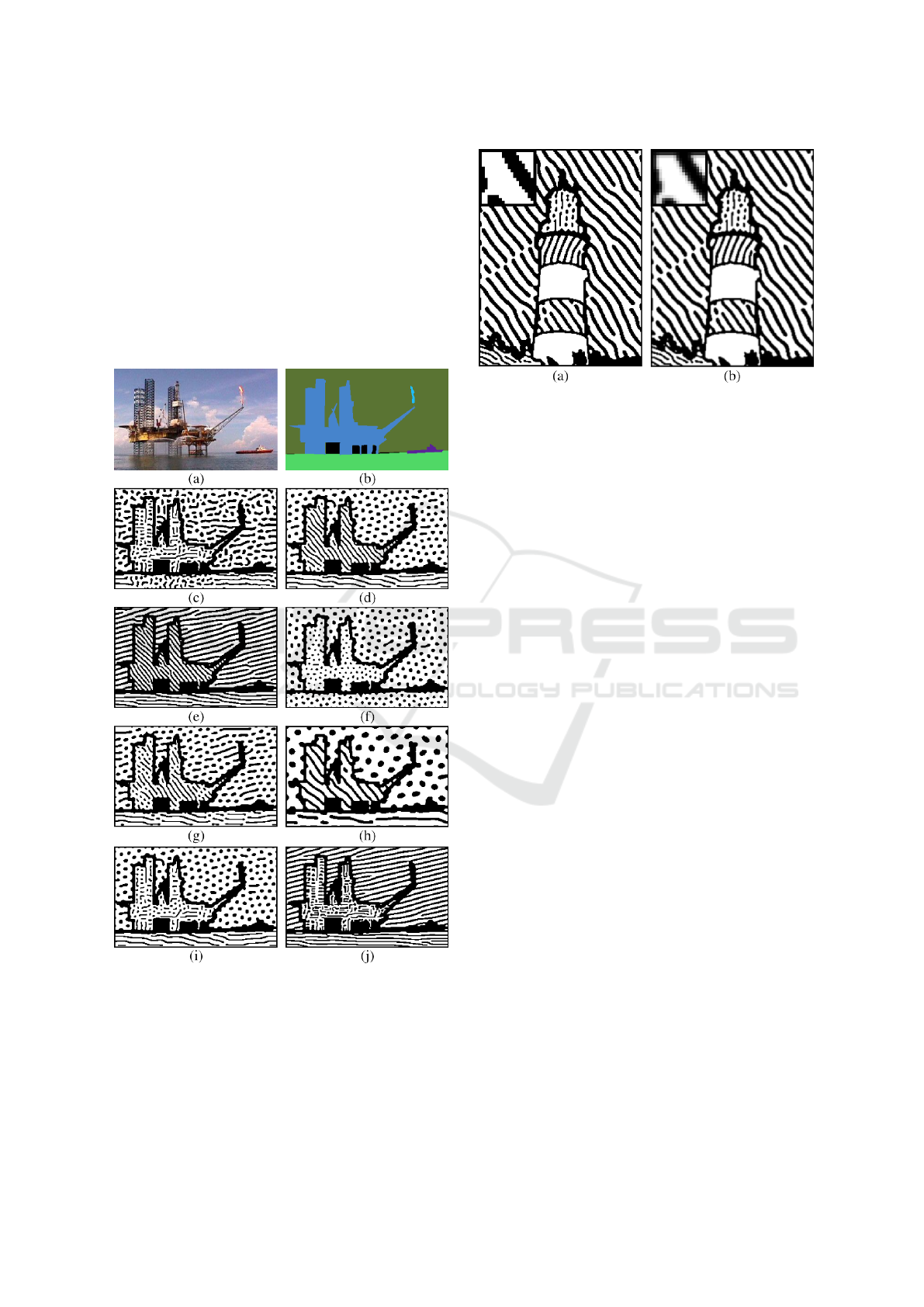
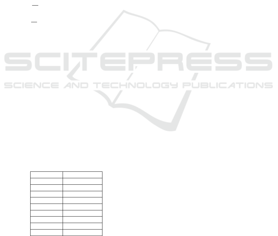
Fig. 3 illustrates the flexibility of our system. For
the same input image, many woodcut variations are
possible by adjusting the parameters. Different re-
gions can present distinct patterns, which eases the
identification of image parts (Figs. 3d and 7). Figs.
3e and 3f show homogeneous patterns (stripes and
spots, respectively) due to setting an unique value for
δ in the entire image. By setting a smaller difference
between δ
min
and δ
max
the pattern difference is more
nuanced, although still present, as some regions show
longer stripes than others (Fig. 3g). Reducing the val-
Figure 3: (a) Original image from the ADE20k dataset
(Zhou et al., 2017). (b) Segmentation of the image from
the ADE20k dataset. (c) Result for θ calculated by pixel
(D
bh
= 0.040, D
bv
= 0.020, static visualization). (d) Result
using the default value for parameters. (e) Result for δ
max
= 0.5. (f) Result for δ
min
= 1.2 and δ
max
= 1.2. (g) Result
for δ
min
= 0.8 and δ
max
= 1.2. (h) Result for S
min
= 0.002
and S
max
= 0.005. (i) Result for adaptive orientation (with
static visualization). (j) Result for adaptive orientation (D
bh
= 0.040, D
bv
= 0.020, δ
max
= 0.5 and static visualization).
Figure 4: Example of the post-processing smoothing op-
tional step (with k = {1,11, 21} and T
di f f
= 10.0). In the
top left, a close-up of the result. (a) Result without smooth-
ing. (b) Result with smoothing.
ues for S makes the stripes and spots bigger (Figs. 3h
and 8). When allowing each pixel to have their own
stroke orientation θ, it is possible to preserve details
of the original image from inside the regions (Figs.
3c, 9, 11 and 12). Adaptive orientation can only be
used on specific parts of the image, allowing detail
preservation for the most detailed regions while other
regions have a more consistent single pattern (Figs.
3i, 3j, 6b and 10).
Fig. 6 shows the result for different border widths,
calculated in the start of the preprocessing step. It
should be noted that orientation angle for regions
where θ was calculated by region suffered some al-
terations among these results, due to the dilating pro-
cess changing which was the brightest pixel from the
region limit.
Fig. 4 compares the result with and without the
optional smoothing filter. On one hand, smoothing
filter reduces the aliasing, but the image seems a bit
blurred. Some of our user-defined parameters did not
yield interesting results, so we keep them fixed for all
our simulations, such as T
low
, T
high
, D
ah
, D
av
, t, M
white
and M
black
.
Validation is a difficult task in the general area
of NPR (Isenberg, 2013). A quantitative evaluation
is hard since there are no specific attributes that can
be measured and compared. We perform a qualita-
tive comparison against the previous results address-
ing woodcuts known in the literature, using a light-
house image used in (Mello et al., 2007) and (Li and
Xu, 2015) (Fig. 2a); to test this image, we did a
manual segmentation over it (Fig. 2b). Comparing
with Mello’s work (Fig. 5a), our results (Fig. 5e
and 5f) have a different appearance, with directional
stripes resembling actual strokes, expanding the range
of styles which can be generated. On the other hand,
Reaction-diffusion Woodcuts
95
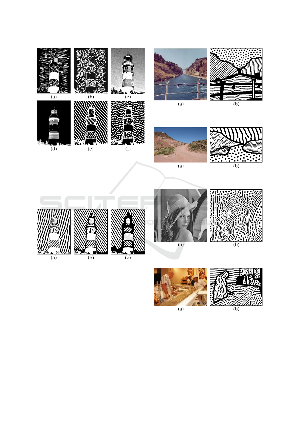
Figure 5: Comparison between different methods for gen-
erating woodcuts (for Fig. 2a). (a) Mello’s result (Mello
et al., 2007). (b) Li’s result (Li and Xu, 2016). (c) Sim-
plify 3 Preset List (Photoshop plugin) result for the Wood
Carving option (Topaz Labs, 2018). (d) Result of a GIMP
pipeline to generate a woodcut-like image (Welch, 2018).
(e) Our result (with k = {1,11,21}, T
di f f
= 10.0 and in-
verted colors). (f) Our result for θ calculated by pixel (with
k = {1,11,21}, T
di f f
= 10.0, D
bh
= 0.040, D
bv
= 0.020,
static visualization, and inverted colors).
Figure 6: Comparison between different border widths, ob-
tained by varying the value of n
dilate
(for Fig. 2a with
k = {1,11,21}, T
di f f
= 10.0, D
bh
= 0.040, D
bv
= 0.020,
static visualization and adaptive orientation). (a) Result
for n
dilate
= 0. (b) Result for n
dilate
= 1. (c) Result for
n
dilate
= 2.
Li’s work (Li and Xu, 2016) is also aesthetically ap-
pealing (Fig. 5b), representing a different woodcut
style than ours (since it intends to simulate the Yun-
nan Out-of-Print woodcut, a tradition Chinese style).
We also tested some image processing tools such as
Adobe Photoshop and GIMP (Figs 5c and 5d), which
did not yield images resembling actual wood carv-
ings.
It should be noted that many of our woodcuts
have an appearance similar to typical Brazilian North-
east woodcuts (as Fig. 12, for example), which are
Figure 7: Results from a channel image from the ADE20K
dataset. (a) Original image (Zhou et al., 2017). (b) Result-
ing woodcut.
Figure 8: Results from a desert road image from the
ADE20K dataset. (a) Original image (Zhou et al., 2017).
(b) Resulting woodcut (with S
min
= 0.002 and S
max
= 0.018).
Figure 9: Results using Lenna. (a) Original image. (b) Re-
sulting woodcut (without segmentation, and with S and θ
calculated by pixel).
Figure 10: Results from a delicatessen image from the
ADE20K dataset. (a) Original image (Zhou et al., 2017).
(b) Resulting woodcut (with T
size
= 300, adaptive orienta-
tion, T
di f f
= 10.0, D
bh
= 0.040, D
bv
= 0.020 and static visu-
alization).
characterized by an abstract form, a black-and-white
coloration (including areas with flat black and white
color), and the usage of lines and points to express
GRAPP 2019 - 14th International Conference on Computer Graphics Theory and Applications
96
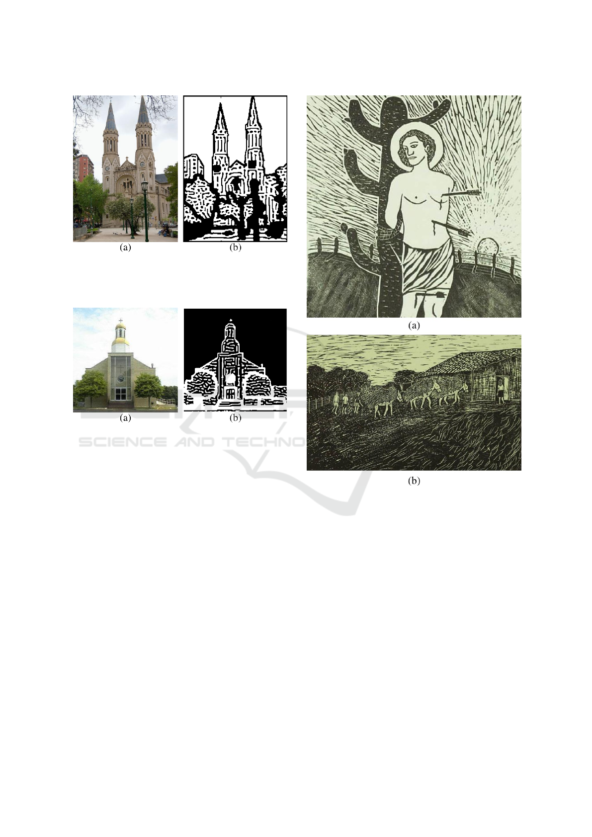
Figure 11: Results from a church image from the ADE20K
dataset. (a) Original image (Zhou et al., 2017). (b) Result-
ing woodcut (with θ by pixel, D
bh
= 0.040, D
bv
= 0.020 and
static visualization).
Figure 12: Results from a church image from the ADE20K
dataset. (a) Original image (Zhou et al., 2017). (b) Result-
ing woodcut (with θ by pixel, D
bh
= 0.040, D
bv
= 0.020,
static visualization, and inverted colors).
different textures (Fig. 13, for example).
A limitation of our work is that, due to the nature
of RD processes as the distribution of chemical sub-
stances forming waves of larger or smaller concen-
tration, white and black stripes have more or less the
same relative width proportion, so it is not possible to
vary the spacing of strokes. Another limitation is the
inability to have lines crossing each others (as in the
walls of the house in Fig. 13b) In actual woodcuts,
strokes are usually more regular than our wave-like
stripes, and tend to be longer, without breaking in the
middle as sometimes the reaction-diffusion stripes do.
For our simulations, we used an Ubuntu PC with
4 GB of RAM memory and an Intel Core 2 Duo pro-
cessor (2.80 GHz x2). For Fig. 3(d), for instance, our
system took a total of 221 seconds, being 15sec for
the preprocessing (mainly for the computation of S
values), 201sec for the RD simulation, and 5sec for
post-processing. It should be taken into account that
this work is a proof of concept, so our focus was not
on code optimization. Also, for many cases, the pat-
Figure 13: Actual woodcuts from the Brazilian Northeast
Region. (a) (Francorli, 2018), (b) (Gonzaga, 2018).
tern was settled before t = 16,000 iterations. To bet-
ter analyze the process, the RD system shows the im-
age being generated on real time, which increases the
computation burden.
5 CONCLUSIONS
We presented a technique to synthesize a woodcut im-
age by using RD. To do that, first we apply a prepro-
cessing step on the input image where we compute
information regarding the detail level and the orien-
tation of strokes, generating a parameter map. Then
we run a RD system over this parameter map. Last, a
post-processing step is done in order to remove noise
and binarize the image, resulting into a black and
white woodcut, which holds similarity to some styles
Reaction-diffusion Woodcuts
97

of actual woodcuts. Our work shows that RD has a
good potential for artistic ends.
To improve our woodcut generating system, we
intend to add noise to better simulate the appearance
of wood grain in our final woodcuts. Computational
efficiency can be improved by setting a stabilization
condition for the RD system, so the system will not
need to run the entire t steps after being stabilized
into a pattern. Finally, we plan to perform a quali-
tative evaluation of our woodcut images, to properly
validate the quality of our results, using the method-
ologies described by (Isenberg, 2013).
ACKNOWLEDGEMENTS
This study was partially financed by the Coordenac¸
˜
ao
de Aperfeic¸oamento de Pessoal de N
´
ıvel Superior -
Brasil (CAPES) - Finance Code 001
REFERENCES
Bard, J. (1981). A model for generating aspects of zebra and
other mammalian coat patterns. Journal of Theoretical
Biology, 93(2):363–385.
Bard, J. and Lauder, I. (1974). How well does turing’s the-
ory of morphogenesis work? Journal of Theoretical
Biology, 45(2):501–531.
Barros, R. S. and Walter, M. (2017). Synthesis of human
skin pigmentation disorders. In Computer Graphics
Forum, volume 36, pages 330–344. Wiley Online Li-
brary.
Chi, M.-T., Liu, W.-C., and Hsu, S.-H. (2016). Image styl-
ization using anisotropic reaction diffusion. The Vi-
sual Computer, 32(12):1549–1561.
DiVerdi, S., Krishnaswamy, A., Mch, R., and Ito, D. (2013).
Painting with polygons: A procedural watercolor en-
gine. IEEE Transactions on Visualization and Com-
puter Graphics, 19(5):723–735.
Francorli (2018). S
˜
ao Sebasti
˜
ao. Available at the Centro
Nacional de Folclore e Cultura Popular (CNFCP) site:
http://www.cnfcp.gov.br/interna.php?ID Secao=64.
[Online; accessed December 10th 2018].
Gonzaga, J. L. (2018). Meninos Cambiteiros.
Available at the Centro Nacional de Fol-
clore e Cultura Popular (CNFCP) site:
http://www.cnfcp.gov.br/interna.php?ID Secao=64.
[Online; accessed December 10th 2018].
Haeberli, P. (1990). Paint by numbers: Abstract image rep-
resentations. In ACM SIGGRAPH computer graphics,
volume 24, pages 207–214. ACM.
Hegde, S., Gatzidis, C., and Tian, F. (2013). Painterly ren-
dering techniques: a state-of-the-art review of current
approaches. Journal of Visualization and Computer
Animation, 24:43–64.
Hertzmann, A. (1998). Painterly rendering with curved
brush strokes of multiple sizes. In Proceedings of the
25th annual conference on Computer graphics and in-
teractive techniques, pages 453–460. ACM.
Isenberg, T. (2013). Evaluating and validating non-
photorealistic and illustrative rendering. In Image
and video-based artistic stylisation, pages 311–331.
Springer.
Jho, C.-W. and Lee, W.-H. (2017). Real-time tonal depic-
tion method by reaction–diffusion mask. Journal of
Real-Time Image Processing, 13(3):591–598.
Kider Jr., J. T., Raja, S., and Badler, N. I. (2011). Fruit
senescence and decay simulation. Computer Graphics
Forum, 30(2):257–266.
Kyprianidis, J. E., Collomosse, J., Wang, T., and Isenberg,
T. (2013). State of the “art”: A taxonomy of artis-
tic stylization techniques for images and video. IEEE
transactions on visualization and computer graphics,
19(5):866–885.
Lai, Y.-K. and Rosin, P. L. (2013). Non-photorealistic
rendering with reduced colour palettes. In Image
and Video-Based Artistic Stylisation, pages 211–236.
Springer.
Li, J. and Xu, D. (2015). A scores based rendering for yun-
nan out-of-print woodcut. In Computer-Aided Design
and Computer Graphics (CAD/Graphics), 2015 14th
International Conference on, pages 214–215. IEEE.
Li, J. and Xu, D. (2016). Image stylization for yunnan out-
of-print woodcut through virtual carving and printing.
In International Conference on Technologies for E-
Learning and Digital Entertainment, pages 212–223.
Springer.
Lu, C., Xu, L., and Jia, J. (2012). Combining sketch and
tone for pencil drawing production. In Proceedings of
the Symposium on Non-Photorealistic Animation and
Rendering, NPAR ’12, pages 65–73, Goslar Germany,
Germany. Eurographics Association.
Mello, V., Jung, C. R., and Walter, M. (2007). Virtual wood-
cuts from images. In Proceedings of the 5th interna-
tional conference on Computer graphics and interac-
tive techniques in Australia and Southeast Asia, pages
103–109. ACM.
Mizuno, S., Kobayashi, D., Okada, M., Toriwaki, J., and
Yamamoto, S. (2006). Creating a virtual wooden
sculpture and a woodblock print with a pressure sen-
sitive pen and a tablet. Forma, 21(1):49–65.
Otsu, N. (1979). A threshold selection method from gray-
level histograms. IEEE transactions on systems, man,
and cybernetics, 9(1):62–66.
Strothotte, T. and Schlechtweg, S. (2002). Non-
photorealistic computer graphics: modeling, render-
ing, and animation. Morgan Kaufmann.
Stuyck, T., Da, F., Hadap, S., and Dutr
´
e, P. (2017). Real-
time oil painting on mobile hardware. In Computer
Graphics Forum, volume 36, pages 69–79. Wiley On-
line Library.
Topaz Labs (2018). Simplify plugin for photoshop. URL:
https://topazlabs.com/simplify/. [Online; accessed
September 23th 2018].
Turing, A. M. (1952). The chemical basis of morphogene-
sis. Phil. Trans. R. Soc. Lond. B, 237(641):37–72.
Turk, G. (1991). Generating textures for arbitrary surfaces
using reaction-diffusion. In Computer Graphics (Pro-
ceedings of SIGGRAPH 91), pages 289–298.
GRAPP 2019 - 14th International Conference on Computer Graphics Theory and Applications
98

Wang, M., Wang, B., Fei, Y., Qian, K., Wang, W., Chen,
J., and Yong, J. (2014). Towards photo watercoloriza-
tion with artistic verisimilitude. IEEE Transactions on
Visualization and Computer Graphics, 20(10):1451–
1460.
Welch, M. (2018). Gimp tips - woodcut. URL:
http://www.squaregear.net/gimptips/wood.shtml.
[Online; accessed September 23th 2018].
Winnem
¨
oller, H. (2011). Xdog: advanced image styliza-
tion with extended difference-of-gaussians. In Pro-
ceedings of the ACM SIGGRAPH/Eurographics Sym-
posium on Non-Photorealistic Animation and Render-
ing, pages 147–156. ACM.
Witkin, A. and Kass, M. (1991). Reaction-diffusion tex-
tures. In Computer Graphics (Proceedings of SIG-
GRAPH 91), pages 299–308.
Zhou, B., Zhao, H., Puig, X., Fidler, S., Barriuso, A., and
Torralba, A. (2017). Scene parsing through ade20k
dataset. In Proceedings of the IEEE Conference on
Computer Vision and Pattern Recognition, volume 1,
page 4. IEEE.
Reaction-diffusion Woodcuts
99
