
Evaluation of Spatial-Temporal Anomalies in the Analysis of Human
Movement
Rui Varandas
1
, Duarte Folgado
1
and Hugo Gamboa
2
1
Associac¸
˜
ao Fraunhofer Portugal Research, Rua Alfredo Allen 455/461, Porto, Portugal
2
Laborat
´
orio de Instrumentac¸
˜
ao, Engenharia Biom
´
edica e F
´
ısica da Radiac¸
˜
ao (LIBPhys-UNL), Departamento de F
´
ısica,
Faculdade de Ci
ˆ
encias e Tecnologia, FCT, Universidade Nova de Lisboa, 2829-516 Caparica, Portugal
Keywords:
Time Series, Anomaly Detection, Human Motion, Unsupervised Learning, Industry.
Abstract:
In industrial contexts, the performed tasks consist of sets of predetermined movements that are continuously
repeated. The execution of improper movements and the existence of events that might prejudice the produc-
tive system are regarded as anomalies. In this work, it is proposed a framework capable of detecting anomalies
in generic repetitive time series, adequate to handle human motion from industrial scenarios. The proposed
framework consists of (1) a new unsupervised segmentation algorithm; (2) feature extraction, selection and di-
mensionality reduction; (3) unsupervised classification based on Density-Based Spatial Clustering Algorithm
for applications with Noise. The proposed solution was applied in four different datasets. The yielded results
demonstrated that anomaly detection in human motion is possible with an accuracy of 73±19%, specificity of
74 ± 21% and sensitivity of 74 ± 35%, and also that the developed framework is generic and may be applied
in general repetitive time series with little adaptation effort for different domains.
1 INTRODUCTION
Anomalies consist of events that do not properly con-
form to the expected behaviour of a given dataset.
Anomaly detection has been widely studied and ap-
plied in diverse domains, such as electrocardiogram
(ECG) signals, video from surveillance cameras and
stock markets (Chandola et al., 2009). The impor-
tance of anomaly detection lies in the fact that such
events are usually associated with defective processes
that might cause failures in the future. Taking the ex-
ample of ECG signals, anomalies might be associated
to cardiac arrhythmias, which may be an early or ac-
tual indicative of heart diseases.
The increasing demands of Industry 4.0 require
highly customised products and adaptive manufactur-
ing systems. The detection of unplanned or planned
anomalies in Human movement on industrial produc-
tion lines is a valuable asset for production control
systems. This information is able to deliver intelli-
gence regarding occurrences that might prejudice the
productive process, reducing the overall productivity
and compromising ergonomics and safety at work.
Furthermore, the monitoring of human motion in such
environments allows to detect predetermined move-
ments that the operators are instructed to follow in or-
der to improve production and ergonomic conditions.
Therefore, an anomaly may consist of wrongly per-
formed movements, which may prejudice ergonomic
conditions and improve the risk of appearance of mus-
culoskeletal disorders.
The Human movement in Industrial scenarios can
be monitored using inertial sensors, which provide
tridimensional motion information. For each task as-
sociated with a given workstation on a production
line, there is a well-defined method that must be fol-
lowed to accomplish it. However, since methods
vary according to the workstation, the repetitive iner-
tial data might exhibit different morphologies despite
maintaining the quasi-periodic behaviour.
2 RELATED WORK
Anomaly detection has been the target of extensive
research and various surveys were already published
(Teng, 2010; Chandola et al., 2009).
For instance, HOT SAX is a method based on the
SAX representation, developed in (Thuy et al., 2018),
to find discords which are sequences that are the most
dissimilar to its k nearest neighbours. Therefore, this
algorithm, is able to find anomalies in time series, but
Varandas, R., Folgado, D. and Gamboa, H.
Evaluation of Spatial-Temporal Anomalies in the Analysis of Human Movement.
DOI: 10.5220/0007386701630170
In Proceedings of the 12th International Joint Conference on Biomedical Engineering Systems and Technologies (BIOSTEC 2019), pages 163-170
ISBN: 978-989-758-353-7
Copyright
c
2019 by SCITEPRESS – Science and Technology Publications, Lda. All rights reserved
163

it is necessary to know the number of anomalies to be
found a priori.
In (Ren et al., 2017), it was developed the PAPR
representation method coped with the construction of
a Random Walk model with the intent to search for
anomalous patterns in time series. The proposed al-
gorithm was tested in 14 different real world datasets
and compared with the PAA method, achieving higher
results. While PAA method detected 15 anomalies,
PAPR associated with Random Walk (PAPR-RW) al-
gorithm was able to detect 25 anomalies out of 27,
and so, the sensitivity is approximately 92%.
There are numerous other examples of anomaly
detection in time series, such as, network source data
(Chen and Li, 2011), gait analysis (Cola et al., 2015),
streaming data (Ahmad et al., 2017), ECG signals
(Ren et al., 2017), in which arrhythmias may be
viewed as anomalies, and detection of mental stress
(Huysmans et al., 2018), in which case, stress states
may be considered anomalous.
Most mentioned methods, though being adequate
for particular applications, lack the capability of be-
ing applicable in different domains. Furthermore, the
methods that may be applied to various domains, ei-
ther need high numbers of parameters or the required
parameters are difficult to assess, for example the
number of anomalies to detect.
This work comprises the development of a novel
framework for anomaly detection applied to domain-
independent repetitive time series, requiring a low
number of parameters to be selected and in which, the
parameters have physical meaning, facilitating their
estimation. This approach is indicated in our con-
text, because in manufacture environments, different
workstations involve different methods, which results
in different repetitive patterns. Thus, it is able to
cope with different time series domains with mini-
mum adaptation effort. In order to achieve this, our
work presents two major contributions: (1) a new un-
supervised segmentation algorithm for quasi-periodic
time series, which is able to extract repetitive units
from those time series, and (2) an unsupervised learn-
ing approach that relies on an exhaustive set of fea-
tures to provide anomaly detection. The proposed
framework was validated on 4 datasets from different
domains, comprising both synthetic and real data.
3 PROPOSED APPROACH
Anomalies are data points or groups of data points
that do not conform well to the whole dataset. Given
a time series X = {x
1
, x
2
, ..., x
N
}, it is possible to seg-
ment it in M subsequences as
X = {S
1
, S
2
, ..., S
M
} (1)
where each S
i
, i ∈ {1, 2,..., M} is a subsequence of X
composed of a defined number of data points, that
may vary from segment to segment and each x
t
,t ∈
{1, 2,..., N} is a measurement at instant t, where N is
the total number of data points. Therefore, the time
series may be represented as
X = {{x
1
, ..., x
k
1
}, ..., {x
k
M−1
+1
, ..., x
k
M
}} (2)
The analysis of each subsequence is usually accom-
plished using a cost function that may indicate dis-
tance or density, for instance. Thus, a subsequence S
i
is anomalous if
f (S
i
, S
j
) > δ ∀ j ∈ [1 : M] (3)
where S
j
may correspond to all subsequences except
S
i
, a model of a normal pattern, or a set of rules that
S
i
must obey to be considered a normal segment. The
value of f (S
i
, S
j
) is the anomaly score, which can be
considered the anomaly degree of S
i
and expresses the
amount of dissimilarity to the model. The definition
of the threshold, δ, controls the sensitivity of each al-
gorithm.
The proposed approach, illustrated in Figure 1,
starts with the application of an unsupervised seg-
mentation algorithm used to extract each cycle from
a repetitive time series. Then, each extracted cycle is
represented by a set of features, followed by a process
of dimensionality reduction using Principal Compo-
nent Analysis. Finally, the transformed feature vector
will be the input for a density based clustering algo-
rithm - DBSCAN.
Figure 1: Diagram of the proposed approach.
3.1 Unsupervised Segmentation
In order to extract cycles from generic repetitive time
series, it was developed a new unsupervised segmen-
tation algorithm, capable of segment time series with-
out prior knowledge about their morphology, period
of repetition or number of cycles, hence, it is consid-
ered dictionary-free.
The developed algorithm is divided into two sep-
arate parts. The first part consists of iteratively seg-
menting a given time series in shorter portions, in a
BIOSIGNALS 2019 - 12th International Conference on Bio-inspired Systems and Signal Processing
164

top-down fashion. Starting with k segments, in which
its limits are constrained to be local minima in a spec-
ified range, the progression of the number of itera-
tions results in an increase of the number of segments.
Then, each segment is represented by its mean value,
thus, each iteration is associated with the set of means
of its segments. Each iteration is then represented by
the standard deviation of the set of means.
The main assumption is that in an ideal cyclic sig-
nal, the mean of each cycle is identical to the rest,
therefore, each value in the set of means is equal to
the average value of the set of means, leading to a
standard deviation of 0 (
¯
S
1
=
¯
S
2
= ... =
¯
S
M
=
¯
S
a
=⇒
σ
a
= 0, where
¯
S
i
, i ∈ {1, ..., M} are the mean values
of each subsequence of a given iteration a,
¯
S
a
is the
mean value of the set of means of iteration a and σ
a
is the standard deviation of the set of means of the
corresponding iteration).
The second part of the developed algorithm is
based on the function of standard deviation vs iter-
ation. The iterations correspondent to local minima
of that function, depicted in the right pane of Figure
2, are selected, as they correspond to the iterations
in which the value of standard deviation decreases,
which means that the segments are more similar.
With those iterations, it is computed the Pearson’s
Correlation Coefficient between each segment and the
rest. Then, each segment is represented by the mean
value of those coefficients and each iteration is repre-
sented by the mean of the representation of its cycles.
Hence, the value that represents each iteration is
restricted to [−1, 1]. The selection of the correct seg-
mentation is based on this value and corresponds to
the iteration with the highest value, meaning that most
segments are highly correlated to all others.
3.2 Feature Extraction and
Dimensionality Reduction
In this work, a comprehensive range of statistical fea-
tures, representation transforms and comparison met-
rics, was used and is summarised in Table 1.
While statistical features and representation trans-
forms are applied for representing each subsequence,
comparison metrics are used to compare each subse-
quence to the total number of subsequences of the
time series. Anomalous subsequences will have a
higher dissimilarity to normal instances, while the
normal subsequences will have a high similarity to
normal instances.
Following feature extraction, the set of features
selected by the user are scaled using a z-score normal-
isation and then transformed by the computation of its
Principal Components, and only the components with
Table 1: Statistical features, representation transforms and
comparison metrics used in this work.
Statistical Features Representation Transforms Comparison Metrics
- Mean Value
- Standard Deviation
- Minimum Value
- Maximum Value
- Inter-Quartile
Range (IQR)
- Number of Peaks
- Median
- Kurtosis
- Skewness
- Duration
-
Linear Regression
(slope and y-intercept)
- Zero Crossing Rate
- Polarity
- Cumulative Summation
- Histogram
- Fourier Transform
- Wavelet Transform
- Principal Component
Analysis Transform
- Independent Component
Analysis Transform
- PAA in the Amplitude
Domain (AD-PAA)
(Ren et al., 2018)
- PAPR (Ren et al., 2017)
- Subsegment Analysis
- Euclidean Distance
- Dynamic Time
Warping Distance
(DTW)
- Time Alignment
Measurement (TAM)
(Folgado et al., 2018)
- Pearson’s Correlation
Coefficient (PCC)
- Cosine Similarity
variance higher than 0,95 are kept for clustering and
classification.
3.3 Clustering and Classification
After feature extraction and dimensionality reduction,
the resulting set of features is introduced as the input
for an unsupervised clustering algorithm - DBSCAN
(Ester et al., 1996).
In order to cluster data points, DBSCAN takes two
hyper-parameters, ε and θ. Based in those parameters,
there are three types of data points: core points, which
are the points that have, at least, a number of θ data
points within a range of ε; density-reachable points,
which are points that belong to the neighbourhood of
a core point, that is, are at a distance lower than ε to a
core point, but do not have a number of θ data points
within ε; noise, which are the points that do not have a
number of θ data points within ε and are not density-
reachable points.
DBSCAN is able to cluster data based on its den-
sity, but it does not classify each data point. The
classification was performed based on the follow-
ing considerations: given that the input to the algo-
rithm are the features extracted and transformed from
each segment representing the samples, if the num-
ber of segments considered to be anomalous is higher
than the number of segments classified as normal, the
value of ε increases by 10% and the clustering pro-
cess is performed again. This process is repeated un-
til the number of normal instances is higher than the
number of anomalous instances. Furthermore, noise
points are always regarded as anomalous and, in cases
when there is more than one cluster, only the cluster
with highest number of points is considered normal.
This last consideration is important in cases in which
anomalies may be similar, thus forming clusters of
their own, such as arrhythmias in ECG signals.
Evaluation of Spatial-Temporal Anomalies in the Analysis of Human Movement
165
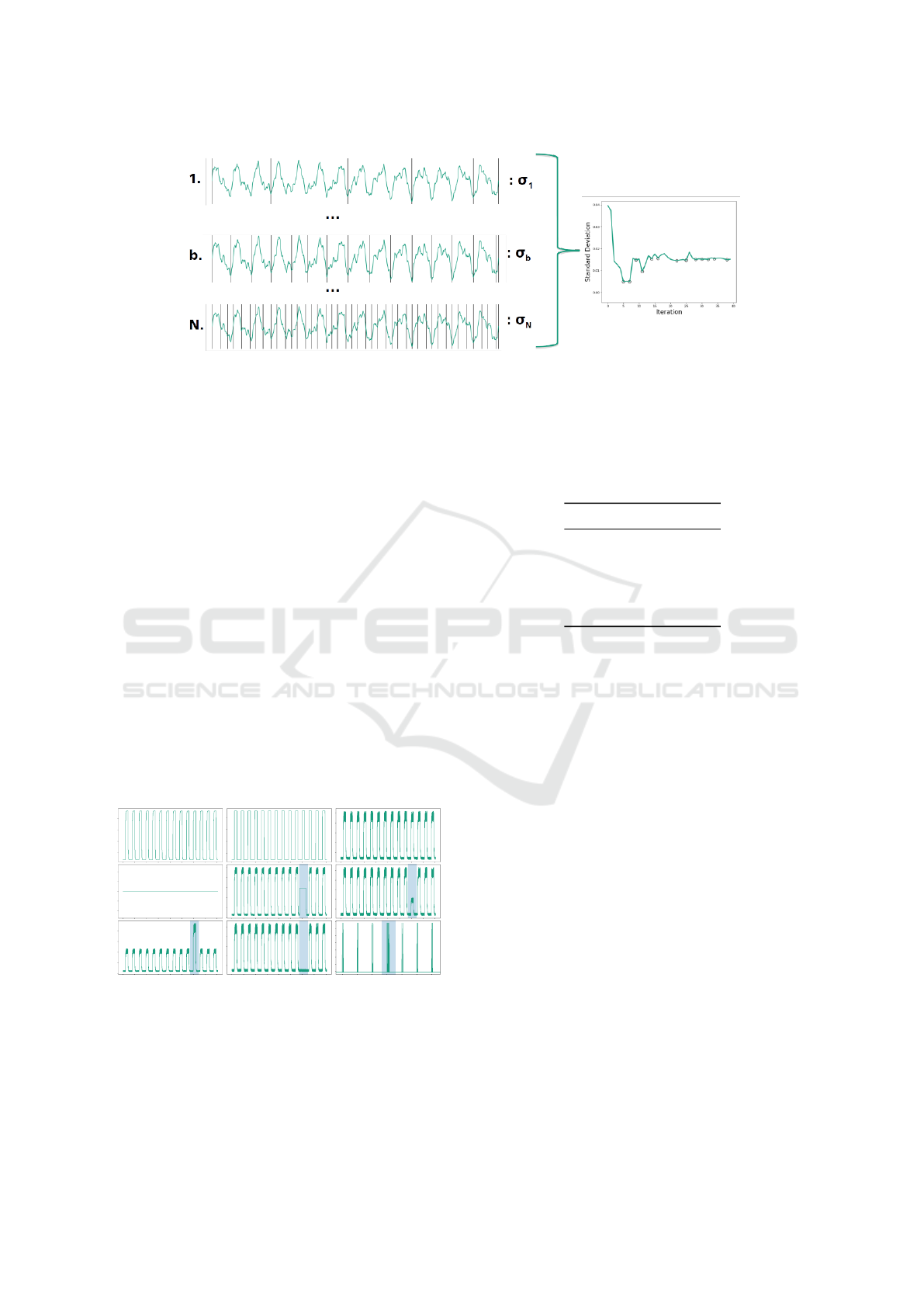
Figure 2: Top-down process of segmentation. Firstly, the time series is segmented in k parts. Then, with each iteration, the
number of segments increases and in each iteration the mean of each segment is computed. Each iteration is represented by
the standard deviation of the set of means of its segments forming a curve such as in the image in right. The negative inflexion
points are chosen for the rest of the process. Iteration b corresponds to the correct segmentation and N corresponds to the last
iteration.
4 RESULTS
The validation of the proposed framework was made
with resource to four datasets, two synthetic and two
composed of real-world data in order to demonstrate
the potential of minimum effort application to differ-
ent domains.
4.1 Numenta Anomaly Benchmark
The first dataset is composed of 9 artificial signals
from Numenta Anomaly Benchmark (NAB) (Ahmad
et al., 2017), illustrated in Figure 3, which was created
to test an algorithm developed by Numenta, the Hier-
archical Temporal Memory (HTM). Since the dataset
comprises different types of anomalies, we only se-
lected the ones which fulfilled the three assumptions
made by the proposed framework.
Figure 3: Numenta Anomaly Benchmark selected signals.
The four initial signals do not present anomalies and, in the
others, the existing anomalies are identified by blue shades.
The results obtained for this dataset are shown in
Table 2.
These results were obtained using mean, max-
imum, minimum, median, inter-quartile range and
Table 2: Results of anomaly detection using the Numenta
Anomaly Benchmark.
Metric Value (%)
Accuracy 99, 3
Specificity 99, 3
Sensitivity 100, 0
Precision 83, 3
F1 score 90, 9
skewness values as the input vector followed by the
procedures described in Section 3. The choice of the
parameters to use in DBSCAN was performed empir-
ically by observing the results and tuning the param-
eters in order to optimise the achieved results. This is
not ideal, because in real life scenarios it is imprac-
ticable to tune the parameters to new signals without
prior knowledge about them. Nevertheless, the pa-
rameters are the same for all signals: θ = 5; ε = 5.
The results show an overfitting scenario due to
the optimisation of the parameters that took into ac-
count all signals. Nevertheless, it is important to point
out that the accuracy is not a good metric to assess
the quality of classification in an unbalanced dataset,
which contains a considerate higher number of nor-
mal segments than anomalous. For example, in the
considered dataset, there are 147 segments and only
5 of them are anomalous. Thus, classifying all seg-
ments as normal, would give an accuracy of 96,6%,
but the classifier would be useless for anomaly de-
tection. Thus, the most appropriate metrics to study
such scenarios are sensitivity, precision and F1 score.
In this case, all metrics show high results except for
precision, because there was 1 false positive, mean-
ing that 5 positives were correctly classified among 6
detected positives.
BIOSIGNALS 2019 - 12th International Conference on Bio-inspired Systems and Signal Processing
166

4.2 Pseudo Periodic Synthetic Time
Series
The Pseudo Periodic Synthetic Time Series dataset
was made publicly available by the Center for Ma-
chine Learning and Intelligent Systems of the Bren
School of Information and Computer Science of the
University of California (Dheeru and Karra Taniski-
dou, 2017). It is composed of 10 artificial signals
composed of 100.000 data points each. These signals
are repetitive, but the cycles are not exactly alike.
These facts make this dataset suitable for testing
the proposed framework, but there is a crucial as-
pect lacking to these signals, which is the presence of
anomalies. Thus, it was generated a set of synthetic
anomalies on amplitude (e.g. noise addition, multipli-
cation by scale vector) and temporal (e.g. nonlinear
temporal distortion) domains. Those anomalies were
randomly introduced in the dataset in a controlled
fashion. This procedure resulted in data augmentation
from 10 to 500 signals, being able to generate a wide
range of different anomaly types in different instants
of the signal.
The results are presented in Table 3. In order
to minimise the influence of overfitting, the hyper-
parameter optimisation was only applied to a small
percentage of data. Therefore, in the validation step,
the majority of data being used was never been sub-
ject to the optimisation procedure. Although this pro-
cedure reduces metric performance, it is more appro-
priate and allows to understand the full extension of
application in real scenarios. The best results were
obtained using the details of the wavelet transform,
in which the mother wavelet was chosen to be of the
family of Daubechies of third order, using θ = 5; ε =
0, 001.
Table 3: Results (mean ± standard deviation) for pseudo-
periodic signals dataset.
Metric Value (%)
Accuracy 91, 6 ±5, 8
Specificity 91, 9 ± 5, 2
Sensitivity 88 ± 28
Precision 52 ± 19
F1 score 64 ± 23
The results are lower than those obtained for NAB
dataset. This is due to the fact that the anomalies
are not as explicit as the ones in NAB and the fact
that hyper-parameter tuning was performed on a small
percentage of data. Specifically, the value of pre-
cision of 52% is low due to the fact that anomalies
may be spread across segments, but could not occupy
a whole segment. Thus, given that the classification
was made in terms of segments, a segment containing
an anomaly could have normal parts, which would be
wrongly classified and are considered false positives,
thus reducing the precision.
However, the results are more representative in
terms of generalisation, which is an essential charac-
teristic of machine learning applications.
4.3 MIT BIH Arrhythmia Database
MIT BIH arrhythmia database (Goldberger et al.,
2000) is a dataset composed of real world ECG
recordings acquired in ambulatory. Electrocardiog-
raphy signals represent the measurement of the elec-
trical pulse that propagates through the cardiac mus-
cle in order to stimulate it, resulting on its normal be-
haviour, which enables the entry and exit of blood to
and from the heart. This normal behaviour may be af-
fected by various factors, resulting in the existence of
cardiac arrhythmias.
The referred dataset is composed of both normal
and anomalous heartbeats totalling 110.000 heart-
beats. Each heartbeat was labelled by two specialist
concerning the position of the R peak and its classifi-
cation regarding the classification in various types of
arrhythmia.
The R peak annotations were used to segment the
signals in order to guarantee a correct segmentation.
Therefore, a segment consisted of a portion of a signal
from the R peak less 100 data points until the next R
peak minus 100 points.
Moreover, it was applied a Butterworth band-pass
filter of second order in order to attenuate frequencies
lower than 1 Hz and higher than 20 Hz, enabling to
reduce interference from normal respiratory frequen-
cies, and muscular and digital noise, respectively.
The results are presented in Table 4. The best
features were duration, polarity, linear regression and
maximum value of each heartbeat. Unlike the first
two datasets, and because the number of heartbeats
(cycles) per signal is significantly higher than in the
previous datasets, it was possible to use the k-Nearest
Neighbour (k-NN) curve to estimate ε, used by the
DBSCAN algorithm, automatically for each signal,
given a fixed θ. Thus, using θ = 5, ε was specific
for each signal.
The performance metrics reveal that real world
electrophysiological signals have considerably more
complex structures and in which anomalies may oc-
cur in several forms. These results are representa-
tive about the accuracy score, which is high, but F1-
score is low. This means that, the great majority of
the dataset is correctly classified, but that is because
Evaluation of Spatial-Temporal Anomalies in the Analysis of Human Movement
167

Table 4: Results (mean ± standard deviation) for anomaly
detection for the MIT BIH arrhythmia database.
Metric Value (%)
Accuracy 89 ± 12
Specificity 92 ± 10
Sensitivity 82 ± 30
Precision 41 ± 33
F1 score 44 ± 33
most normal cycles are considered normal, but several
anomalous cycles are wrongly classified, which low-
ers the value of sensitivity. However, it is notable the
low adaptation effort needed to apply the developed
generic framework to such a specific domain such as
ECG signals.
4.4 Human Motion on Industrial
Scenario
Human motion on industrial scenario (HMIS) dataset
was acquired by the authors in a real industrial en-
vironment with resource to a wearable sensor, that
was integrated into bracelets and placed on employ-
ees’ dominant upper member. This placement al-
lowed to monitor the wrist’s movement performed by
each monitored employee, which is relevant once the
tasks performed involve predominantly upper mem-
ber movements.
The sensing device contains an Inertial Measure-
ment Unit (IMU), which measures inertial data with
resource to three sensors: an accelerometer, a gyro-
scope and a magnetometer. The combination of the
three sensors allows a full comprehensive analysis re-
garding the movement of the monitored employee.
Figure 4 shows an example of the measured inertial
data from a single employee. The black vertical lines
indicate the beginning/ending of a work cycle and the
red part is an example of an anomaly in this context,
which corresponds to a significant deviation in terms
of morphology in relation to other cycles (the phe-
nomenon is more evident in magnetometer data).
The device was connected via Bluetooth LE to
a smartphone, where the data was stored. Each
recorded acquisition was annotated in real-time at the
beginning of each new cycle and in every occurrence
of anomalies, allowing to build the ground-truth seg-
mentation and labelling.
The acquired data consists of inertial data orig-
inated by the movements performed by 4 different
workers at 3 different workstations where they were
producing different items. All tasks monitored were
repetitive which made them suitable to be tested with
the developed anomaly detection framework. The
sampling frequency of the acquisitions was approx-
imately 100Hz and the total time of the acquisitions
is around 4 hours and 20 minutes.
Moreover, once the number of cycles per signal
varies widely, it was not possible to use the k-NN
curve directly in order to estimate them. The fol-
lowed approach was inspired by the Leave-One-Out
cross validation that is used to test algorithms in the
presence of a low number of instances. Given N sig-
nals, we calculate the parameters for every signal, ex-
cept the signal under evaluation, with resource to the
k-NN curve and then use the mean value of the es-
timated values for the untested signal. This process
was repeated for each signal allowing for an objective
test without influence from a human observer.
Table 5 summarises the results of anomaly de-
tection using two different methods for time series
segmentation in work cycles: groundtruth annota-
tions and the proposed unsupervised segmentation
algorithm. The results suggest that both methods
have similar performance. The use of the unsuper-
vised segmentation does have significant advantages
on real-world deployment as it does not require user
intervention in the overall process.
Table 5: Influence of unsupervised segmentation on
anomaly detection of human motion inertial data. The re-
sults (mean ± standard deviation) are reported in terms of
percentage (%).
Metrics
Groundtruth
Segmentation
Unsupervised
Segmentation
Accuracy 73 ± 19 71 ± 16
Specificity 75 ± 22 74 ± 18
Sensitivity 52 ± 45 52 ± 36
Precision 18 ± 23 20 ± 24
F1 score 19 ± 25 20 ± 20
Since previous results suggest that it is feasible
to use the unsupervised segmentation algorithm, the
next step consisted of a comprehensive evaluation
of the features used to describe the detected subse-
quences and thus, able to differentiate between nor-
mal and anomalous instances. Table 6 presents the
results obtained using each feature earlier described
in Table 1. The results show that feature selection in-
fluences the outcome of the clustering algorithm.
The achieved results have overall low perfor-
mance in comparison with previous datasets due
to some factors that will be properly discussed.
Firstly, the process for hyper-parameter optimisation
of DBSCAN algorithm was different from previous
datasets. In the NAB and Pseudo Periodic datasets the
hyper-parameters were specified and optimised by the
user; in the MIT BIH arrythmia database they were
BIOSIGNALS 2019 - 12th International Conference on Bio-inspired Systems and Signal Processing
168
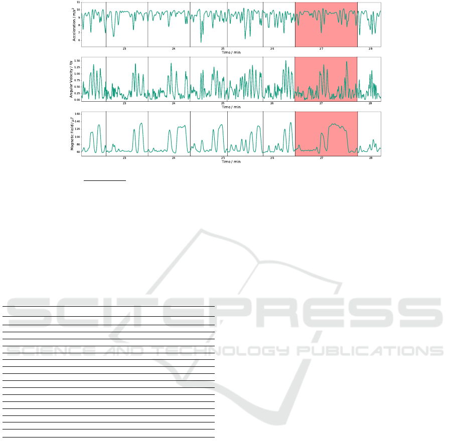
Figure 4: Excerpt of inertial data from a single operator. Each sensor is represented by the magnitude of the three axis x, y
and z (magnitude =
p
x
2
+ y
2
+ z
2
). Each plot corresponds to accelerometer, gyroscope and magnetometer data, respectively,
from top to bottom. The black vertical lines indicate the beginning/ending of a work cycle and the red part corresponds to an
anomaly. The anomaly is more evident in magnetometer data.
Table 6: Influence of feature selection on anomaly detec-
tion of human motion inertial data. The results (mean ±
standard deviation) are reported in terms of percentage (%).
(In the first line, the set of features correspond to the mean,
maximum, minimum, IQR, standard deviation, number of
peaks, median, kurtosis, duration, skewness and linear re-
gression).
Features Accuracy Specificity Sensitivity Precision F1-score
Set of Features 73 ± 19 74±21 74 ± 35 24± 30 30 ± 31
ICA 89 ± 13 96± 11 9 ±28 23 ± 24 6 ± 17
DTW 72 ± 18 77± 21 53 ± 44 15 ± 13 17± 18
TAM 70 ± 19 70± 22 72 ± 41 17 ± 24 23± 28
Fourier Transform 74 ± 16 80 ±19 28 ±34 14 ± 22 13± 17
Polarity 70 ± 17 77 ± 21 38 ± 48 5, 3± 9, 3 8 ± 14
Cumulative Summation 75 ± 20 80 ± 24 28 ± 45 7 ± 12 7 ± 15
Wavelet Approximation 80 ± 23 82 ± 28 40 ±52 20 ± 26 15 ±27
Wavelet Details 65 ± 18 64 ± 22 67 ± 47 14 ± 17 20 ±23
Cosine Similarity 77 ± 21 78 ± 24 53 ± 47 25 ±24 22 ± 28
PCA 75 ± 20 75 ± 25 53 ± 48 20 ±17 19 ± 23
AD-PAA 74 ± 18 75 ± 20 59 ± 47 23 ±29 29 ± 33
Histogram 65 ± 20 65 ± 21 74 ± 32 25 ±30 30 ± 31
Euclidean Distance 73 ± 22 71 ±27 58 ±50 21 ± 17 20 ± 24
Subsegment analysis 67 ± 20 66 ± 21 79 ± 32 18 ±24 25 ± 28
PCC 69 ± 18 76 ± 23 42 ± 47 9 ± 15 6, 6 ±7,3
PAPR 74 ± 18 76 ± 20 64 ± 40 25 ±33 29 ± 33
directly estimated with resource to the k-NN curve.
For the HMIS dataset the parameters were selected by
a Leave-One-Out approach, since the reduced num-
ber of cycles per signal did not allowed to use the k-
NN curve method directly. Secondly, the motion data
was originated from three different workstation which
have different methods and thus, different cyclic be-
haviours and signal morphologies. Therefore, the
mean value of the estimated parameters from different
workstations may not represent the correct value for
neither of them. The most adequate approach would
be to acquire data for a longer period of time in order
to have a dataset composed of longer time series with
a higher number of cycles, which would allow to au-
tomatically estimate the value of parameter ε for each
workstation.
5 CONCLUSIONS
Musculoskeletal disorders are a major concern in
manufacturing environments due to wrongly executed
movements and inadequate postures. Most of the
tasks executed in those environments are repetitive.
Using IMUs to follow human motion, it is possible
to acquire repetitive time series with all the infor-
mation regarding the movements that integrate each
task. Since the method to accomplish each task is
defined with the aim to increase productivity while
preventing the development of musculoskeletal disor-
ders, any significant deviation from it may suggest an
occurrence that hinders the productive process. Those
occurrences appear as anomalies on IMU data. This
high-level information is a valuable asset for produc-
tion control systems, being able to constantly iden-
tify opportunities for continuous refinement of the
production processes in lean manufacturing environ-
ments.
In order to accomplish this requirement, the pro-
posed anomaly detection framework was divided into
three stages: (1) unsupervised segmentation; (2) fea-
ture extraction from the extracted subsegments and
(3) unsupervised classification using DBSCAN.
The validation stage comprised the performance
evaluation on four datasets from different domains,
which proves the requirements were met with regards
of aspiring to build a framework for unsupervised
anomaly detection on repetitive time series.
The results demonstrated that anomaly detection
in generic repetitive time series in an unsupervised
fashion is feasible, however, at the cost of a reduced
performance when compared to domain-specific ap-
Evaluation of Spatial-Temporal Anomalies in the Analysis of Human Movement
169

proaches reviewed in the literature. Notwithstand-
ing, a general approach has the value of being eas-
ily adapted in order to be applied in different do-
mains and in repetitive time series with different mor-
phologies, such as the case of different workstations
in manufacture environments. In human motion in-
dustrial scenarios, which are dominated by repeti-
tive movements, it was possible to detect anomalies
in multivariate time series using accelerometer, gyro-
scope and magnetometer data. However, the detec-
tion depends on the correct feature selection in or-
der to be accurate and still it may present low pre-
cision. Another important aspect is the adequate se-
lection of DBSCAN hyper-parameters. This work
demonstrated that a high volume of data and cycles
are required in order to properly automate the hyper-
parameter selection. For challenges with relatively
low volume of data either the hyper-parameter opti-
misation was achieved by user selection (at the cost
of low generalisation properties despite high perfor-
mance values) or by a Leave-One-Out methodology
which resulted in difficulties to achieve a set of val-
ues which maintain optimal characteristics for a wide
range of signals.
Future work will consist in validating the frame-
work over a more exhaustive volume of data,
which should facilitate the process of proper hyper-
parameter optimisation. Furthermore, this work was
focused on the development of the described anomaly
detection framework, but it would be important to as-
sess the impact of this system in Industrial production
lines in long-term.
ACKNOWLEDGEMENTS
This work was supported by North Portugal Regional
Operational Programme (NORTE 2020), Portugal
2020 and the European Regional Development Fund
(ERDF) from European Union through the project
Symbiotic technology for societal efficiency gains:
Deus ex Machina (DEM) [NORTE-01-0145-FEDER-
000026].
REFERENCES
Ahmad, S., Lavin, A., Purdy, S., and Agha, Z. (2017). Un-
supervised real-time anomaly detection for streaming
data. Neurocomputing, 262:134 – 147. Online Real-
Time Learning Strategies for Data Streams.
Chandola, V., Banerjee, A., and Kumar, V. (2009).
Anomaly Detection: A Survey. ACM Computing Sur-
veys, 41(3):1–58.
Chen, Z. and Li, Y. F. (2011). Anomaly detection based on
enhanced dbscan algorithm. Procedia Engineering,
15:178 – 182. CEIS 2011.
Cola, G., Avvenuti, M., Vecchio, A., Yang, G.-Z., and Lo,
B. P. L. (2015). An on-node processing approach
for anomaly detection in gait. IEEE Sensors Journal,
15:6640–6649.
Dheeru, D. and Karra Taniskidou, E. (2017). UCI machine
learning repository.
Ester, M., Kriegel, H.-P., Sander, J., and Xu, X. (1996).
A density-based algorithm for discovering clusters a
density-based algorithm for discovering clusters in
large spatial databases with noise. In Proceedings of
the Second International Conference on Knowledge
Discovery and Data Mining, KDD’96, pages 226–
231. AAAI Press.
Folgado, D., Barandas, M., Matias, R., Martins, R., Car-
valho, M., and Gamboa, H. (2018). Time Alignment
Measurement for Time Series. Pattern Recognition,
81:268–279.
Goldberger, A. L., Amaral, L. A. N., Glass, L., Hausdorff,
J. M., Ivanov, P. C., Mark, R. G., Mietus, J. E., Moody,
G. B., Peng, C.-K., and Stanley, H. E. (2000). Phys-
iobank, physiotoolkit, and physionet. Circulation,
101(23):e215–e220.
Huysmans, D., Smets, E., Raedt, W. D., Hoof, C. V., Bo-
gaerts, K., Diest, I. V., and Helic, D. (2018). Unsu-
pervised learning for mental stress detection. In Pro-
ceedings of the 11th International Joint Conference
on Biomedical Engineering Systems and Technologies
- Volume 4: BIOSIGNALS, (BIOSTEC 2018), pages
26–35. INSTICC, SciTePress.
Ren, H., Liao, X., Li, Z., and AI-Ahmari, A. (2018).
Anomaly detection using piecewise aggregate approx-
imation in the amplitude domain. Applied Intelli-
gence, 48(5):1097–1110.
Ren, H., Liu, M., Li, Z., and Pedrycz, W. (2017). A Piece-
wise Aggregate Pattern Representation Approach for
Anomaly Detection in Time Series. Knowledge-Based
Systems, 135:29–39.
Teng, M. (2010). Anomaly detection on time series. 2010
IEEE International Conference on Progress in Infor-
matics and Computing, 1:603–608.
Thuy, H. T. T., Anh, D. T., and Chau, V. T. N. (2018).
Comparing three time series segmentation methods
via novel evaluation criteria. In Proceedings - 2017
2nd International Conferences on Information Tech-
nology, Information Systems and Electrical Engineer-
ing, ICITISEE 2017, volume 2018-Janua, pages 171–
176.
BIOSIGNALS 2019 - 12th International Conference on Bio-inspired Systems and Signal Processing
170
