
Clustering Honeybees by Its Daily Activity
Edgar Acuna
1
, Velcy Palomino
2
, Jos´e Agosto
3
, R´emi M´egret
4
, Tugrul Giray
3
, Alberto Prado
5,6
,
C´edric Alaux
5,6
and Yves Le Conte
5,6
1
Department of Mathematical Sciences, University of Puerto Rico, Mayaguez PR 00682, U.S.A.
2
Program in Computing and Information Science and Engineering, University of Puerto Rico, Mayaguez PR 00682, U.S.A.
3
Department of Biology, University of Puerto Rico, Rio Piedras, PR 00990, U.S.A.
4
Department of Computer Science, University of Puerto Rico, Rio Piedras, PR 00990, U.S.A.
5
INRA, UR406 Abeilles & Environnement, Site Agroparc, 84914 Avignon, France
6
UMT PrADE, Site Agroparc, 84914 Avignon, France
alberto.prado-farias@inra.fr, cedric.alaux@inra.fr, yves.le-conte@inra.fr
Keywords:
Clustering, Honeybees Behavior, Data Wrangling, Time Series.
Abstract:
In this work, we analyze the activity of bees starting at 6 days old. The data was collected at the INRA (France)
during 2014 and 2016. The activity is counted according to whether the bees enter or leave the hive. After
data wrangling, we decided to analyze data corresponding to a period of 10 days. We use clustering method to
determine bees with similar activity and to estimate the time during the day when the bees are most active. To
achieve our objective, the data was analyzed in three different time periods in a day. One considering the daily
activity during in two periods: morning and afternoon, then looking at activities in periods of 3 hours from
8:00am to 8:00pm and, finally looking at the activities hourly from 8:00am to 8:00pm. Our study found two
clusters of bees and in one of them clearly the bees activity increased at the day 5. The smaller cluster included
the most active bees representing about 24 percent of the total bees under study. Also, the highest activity of
the bees was registered between 2:00pm until 3:00pm. A Chi-square test shows that there is a combined effect
Treatment× Colony on the clusters formation.
1 INTRODUCTION
This work is part of a larger effort to characterize and
provide tools for the analysis of individual behavior
patterns of honeybees in their natural environment,
i.e. the hives in the field. The goal is to be able to
observe the variations in behavior of individuals in-
stead of reasoning on aggregates and averages at the
population level. In this paper, the bee activity is rep-
resented by the events entering (E) and exiting (S)
the hive. Bees were marked with individual tags and
recognized when passing an optical detector located
at the only entrance of the hive, which can associate
each event with an individual bee based on its tag.
Our hypothesis is that the individual patterns of be-
havior will form clusters of bees with similar activity,
which can inform us on the latent parameters associ-
ated to the individual bees. The categorical features
“Treatment” and “Colony” have not been taken into
account in the clustering task avoiding the use of a
similarity distance involving mixed attributes like the
Gower distance. However, the effect of both features
on the clusters formation is discussed in detail in sec-
tion 3.2. The main goal of this work is to find out
clusters of bees with similar activity.
This paper is organizedas follows: In section 2 the
datasets used and wrangling of the times series data
are detailed. In section 3, the clustering process is
discussed. In section 4, an explanation of the finding
of the time interval with the peak activity is given. Fi-
nally, in the last section, we mention the conclusions
of this work.
2 DATA PREPARATION
2.1 Datasets
In this study, we have considered seven datasets
from experiments with bees carried out at the INRA
(France). The first three datasets are coming from an
598
Acuna, E., Palomino, V., Agosto, J., Mégret, R., Giray, T., Prado, A., Alaux, C. and Conte, Y.
Clustering Honeybees by Its Daily Activity.
DOI: 10.5220/0007387505980604
In Proceedings of the 8th International Conference on Pattern Recognition Applications and Methods (ICPRAM 2019), pages 598-604
ISBN: 978-989-758-351-3
Copyright
c
2019 by SCITEPRESS – Science and Technology Publications, Lda. All rights reser ved

experiment carried out in 2014 by C. Bordier (Bor-
dier et al., 2017). In there, newly emerged bees
were infested with Nosema spores. The behavioral
recording started at age 1. The experiment was repli-
cated 3 times using 3 bee counters (colonies) each
time. All the data are pooled in the same file. In
this work, we have separated it into three datasets.
The recordings started on the following dates : 02-
04-2014(dataset 2014-I) , 14-05-2014 (dataset 2014-
II) and 18-06-2014 (dataset 2014- III). In this experi-
ment, one tag was used more than once. Thus, there
are some tags that appear in dataset 2014-I and dataset
2014-II and even in dataset 2014-III. The remaining
datasets were collected by A. Prado in 2016 (Prado
et al., 2019). Prado used 6 Treatments (5 pesticides
mixture and one control) started at 6 days old. The
experiment was replicated 6 times using 2 bee coun-
ters (colony L and colony M) each time. Recordings
for experiment April 2016 started on April 12 ,2016
and ended on May 1, 2016. In here, this dataset is
named 2016A. The first experiment from June 2016,
included cohort1, started on 31-05-2016 , and cohort2
, started on 13-06-2016. The bees are from colony L
and theirs activity recordings end on July 4, 2016. We
have named as 2016J to the dataset including results
from this experiment. The second experiment from
June 2016 included cohort1, started on 31-05-2016,
and cohort2 , started on 13-06-2016. The bees are
from colony M and recordings end on July 4, 2016.
We have called 2016JB to the dataset containing re-
sults from this experiment. In both experiments 2016J
and 2016JB, the cohort2 has only 21 days of mea-
surements. However, we have found that bee with tag
B4359 from the 2016JB has records in days 8th,10th
and 12th of June. Bee’s activity recordings for the ex-
periment from September, 2016 started at 13-09-2016
and emded on 17-10-2016. However, there are two
bees with recordings as earlier as 08-09-2016. This
dataset is named 2016S. The first rows of a typical
dataset (2016JB) are shown in table 1.
Table 1: First rows of the 2016JB dataset.
Id Date Time BeeID Dir. Trt. Colony
1 31-05-2016 09:42:17 B4826 S mix C M
2 31-05-2016 09:42:27 B4823 S mix C M
3 31-05-2016 09:42:27 B4823 E mix C M
4 31-05-2016 09:42:45 B4826 E mix C M
5 31-05-2016 10:49:16 B5113 S Control M
6 31-05-2016 10:54:19 B5113 E Control M
7 31-05-2016 10:54:53 B5113 S Control M
8 31-05-2016 10:56:11 B5113 E Control M
An exhaustive report of the data recollection can
be found in (Prado et al., 2019).
In this work, we are only interested in the bee
activity with respect to either entering (E) or exiting
(S) the hive. The features “Treatment” and “Colony”
have not been taken into account in the clustering task
avoiding the use of a similarity distance involving
mixed attributes like the Gower distance. However,
after the clustering task, we have used both attributes
to explain the clusters formed. Our goal is to find out
clusters of bees with similar activity. This paper is or-
ganized as follows: In section 2 the wrangling of the
times series data is detailed, in section 3, the cluster-
ing process is discussed, in section 4 an explanation
of the finding of the time interval with the highest ac-
tivity is given, finally in the last section we mention
the conclusions of our work.
2.2 Data Wrangling
In order to have a more accurate clustering process,
we have cleanup the data by considering only bees
with more than 10 activities, somehow equivalent to
having more than 5 trips (see Table 2, column 4). All
the datasets have miss detections for direction values,
since several SS (S=Exit) or EE (E=Enter) sequences
for a given bee appear recorded. These can be fixed
but up to certain amount. It is not recommended to fix
more than 30 percent of missed detection since bias
will be generated (see Table 2,column 5). However,
in this paper we have not cleanup miss detection in
the collected data, since we are interestred in the bee
activity regardless if it is an entering or an exiting.
Table 2: The number of bees per experiment, number of
recording days per experiment, number of bees to be con-
sidered for the clustering processing and the number of bees
for which miss detected data can be fixed.
Exp Total number
Days of
Recording
More than
5 trips
less than 30 percent of
missdetection
2014-I 300 34 219 186
2014-II 300 29 185 115
2014-III 300 28 220 174
2016J 740 35/21 544 513
2016JB 691 35/21 490 423
2016A 251 20 144 125
2016S 239 34 203 159
We have merged datasets 2016J and 2016JB since
bees’ activities included in these two datasets were
recorded by the same time calendar. In total, there
are 1431 bees, the activity recording of 786 of them
started on May 31, 2016 (first cohort) and the record-
ing of the remaining 645 started on June 13, 2016
(second cohort) . After removing the bees with less
than 5 trips (10 activities) the number of bees is re-
duced to 1034. The Bee B4359 was discarded for
inconsistency in its recordings as mentioned in sec-
tion 2.1. Thus, only 1033 bees are considered in this
work. From these, 572 bees belong to the first cohort
and 461 bees belong to the second cohort.
Clustering Honeybees by Its Daily Activity
599

Table 3: Numbers of bees with similar time duration (given in days) for each dataset.
Exp 0 1 2 3 4 5 6 7 8 9 10 11 12 13 14 15 16 17 18 19 20 21 22 23 24 25
2014-I 7 4 9 9 6 6 10 5 6 11 10 8 6 3 8 12 8 12 9 5 11 11 6 9 3 4
2014-II 2 2 5 7 7 15 14 15 14 17 11 13 8 14 7 6 7 3 5 4 1 2 0 1 0 2
2014-III 2 6 7 21 15 13 7 13 13 18 16 13 13 17 12 6 8 2 5 3 0 3 1 2 2 1
2016A 1 14 10 11 13 8 5 3 12 7 7 5 5 7 10 6 11 8 0 1
2016J 2 8 11 23 31 42 32 42 34 31 42 46 22 24 19 17 30 14 10 11 13 16 3 6 5 0
2016Jb 2 9 14 22 28 16 21 33 32 31 21 32 23 27 23 19 16 17 24 10 3 10 5 11 5 8
2016S 0 7 16 4 12 13 15 19 7 11 14 10 10 11 9 6 2 1 6 8 2 3 2 3 3 2
2.3 Preparing the Data for Clustering
Our goal is to group bees according to similar ac-
tivity. Since clustering must be performed on data
tables with rows of equal length, first, we have to
find out bees with similar time duration of recording.
We cannot cluster bees with different time duration
of recording, say a bee with three days of record-
ing cannot be clustered along a bee with 20 days of
recording, We wrote an R script using the R package
lubridate to find out bees with equal length time of
recordings,using days as measure of time(Grolemund
and Wickham, 2011). This does not mean that we are
looking for bees with activity recorded in the same
days. In fact, one day (24 hours) of recording can in-
volve two days-calendar. In our program, basically
we found the time duration (in hours) for the record-
ings of a bee and then this time is converted into days.
Finally, we group the bees for their time duration in
days. Table 3 shows the number of bees with simi-
lar number of days recorded for each of the datasets.
Day=0 means that less than 24 hours of bee activ-
ity was recorded, day=1 means that between 24 hours
and 47.99 hours of bee activity was recorded, and so
on. From Table 3, we can notice that there are few
activity recordings after day 25.
In this paper, due to space limitations, for cluster-
ing tasks we have only considered datasets from June
2016. Furthermore, these datasets are the ones with
less inconsistencies. In order to have a large sample
for clustering, after merging the 2016J and 2016JB
datasets, we considered all the bees with 10 or more
days of activities but considering only a time period
of length ten days. For instance, if a bee has a record-
ing of 13 days, we will only took in account its first
10 days of activities. Using this criterion, we ended
up with 382 bees in the first cohort and 188 bees in
cohort 2 as is showed below.
Cohort 1:
Days:Bees 0:2, 1:7 2:9 3:19 4:12 5:18 6:32 7:33
8:32 9:27 10:34 11:42 12:26 13:26 14:25 15:27 16:37
17:23 18:21 19:11 20:21 21:18 22:8 23:17 24:10 25:8
26:8 27:3 28:3 29:2 30:3 31:1 32:5 33:2
Cohort2:
Days: Bees 0:2 1:10 2:16 3:26 4:47 5:40 6:21 7:42
8:34 9:35 10:29 11:36 12:19 13:25 14:17 15:9 16:9
17:8 18:13 19:10 20:5 21 :8
3 PERFORMING THE
CLUSTERING TASK
We have carried out clustering in each June’s cohort
separately. For that, we performed subsetting of the
data file into the two cohorts and count the number of
bee’s activities per hour in each of them. The output
was saved in two csv files one for each cohort. In
the counting of the activity, we have not distinguished
the type of activity, so E and S counts as one activity
each of them. The first six rows of the output file for
cohort1 looks like in Table 4.
Table 4: First six rows of the dataset showing counts of bee
activity per hour.
beesID hour Count
1 B4002 6/1/2016 17:00 2
2 B4002 6/3/2016 15:00 1
3 B4002 6/3/2016 16:00 1
4 B4002 6/5/2016 16:00 2
5 B4002 6/6/2016 15:00 1
6 B4002 6/7/2016 9:00 2
Then, we built a dataframe showing the 382 beees
along the number of theirs activities per day-calendar
but taking into account if the activity was either in the
morning (before 12.00) or in the afternoon (12.00 or
later) from May 31 until June 9. Thus, the dataframe
has 382 rows and 22 columns. The first six rows of
the dataframe are shown in Table 5.
Using outlier detection techniques (Mahalanobis
distance, Local Outlier Factor(LOF) and even cluster-
ing itself), we have detected that bees with tags B4387
and B5134 are clearly outliers (Tan et al., 2005). Both
bees are from colony M. In Figure 1, we compare the
activity of a typical bee (B4013) with the activity of
the two outliers bees. Notice that the outliers bees be-
gan an unsual activity during the mornings starting at
day 5. This highly active bees may represent highly
especilized such as water foragers (Robinson et al.,
ICPRAM 2019 - 8th International Conference on Pattern Recognition Applications and Methods
600
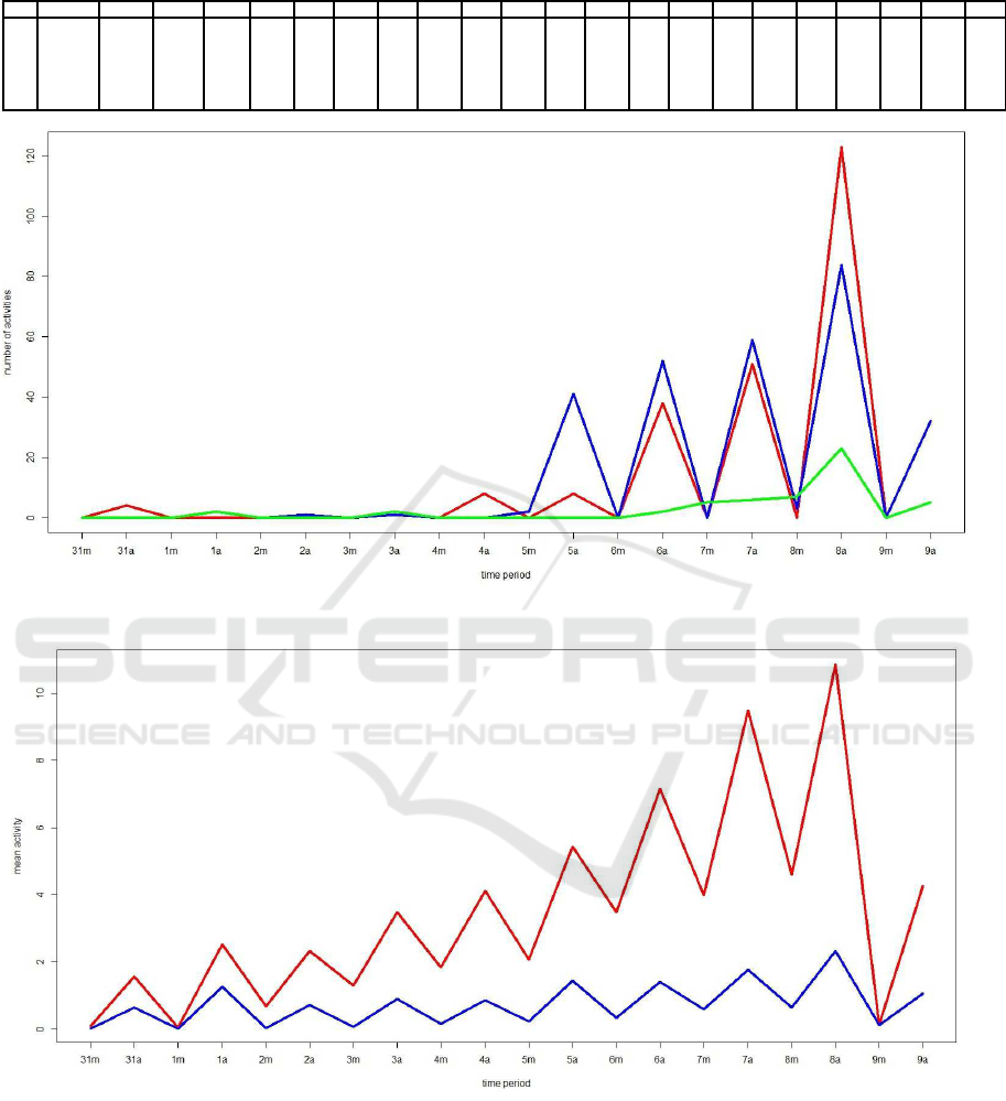
Table 5: Numbers of bees with similar time duration (given in days-calendar.
BeeID Total 31m 31a 1m 1a 2m 2a 3m 3a 4m 4a 5m 5a 6m 6a 7m 7a 8m 8a 9m 9a
1 B4002 32 0 0 0 2 0 0 0 2 0 0 0 2 0 1 2 2 1 2 0 1
2 B4005 226 0 2 0 0 0 4 0 0 0 0 0 2 0 0 0 0 0 2 0 7
3 B4006 161 0 0 0 2 0 0 0 4 0 0 0 1 0 2 0 2 2 2 0 0
4 B4010 77 0 0 0 2 0 0 0 2 0 0 0 4 0 2 1 1 0 32 0 6
5 B4011 97 0 2 0 0 0 2 0 0 0 1 0 3 0 2 0 4 0 4 0 26
6 B4012 50 0 0 0 2 0 0 0 0 0 1 0 1 0 2 2 4 0 5 1 6
Figure 1: Plot to compare the activity of a normal bee (green) with the two outliers bees (B4387 and B5134) in cohort 1.
Figure 2: Plot of bees’ activity means at each time period of the two clusters formed using kmeans.
1984). Therefore, we have excluded this two bees be-
cause it can harm the clustering process, in particular
kmeans, which requires means computation.
To find the groups with similar activity formed
from the 380 bees in cohort 1, we apply two cluster-
ing algorithms: Kmeans, Partitioning around medoids
(PAM) and Agglomerative hierarchical(AGNES) to
the data partly shown in table 5 (Jain and Dubes,
1988). We have evaluated from two up to six clusters.
In Table 6, we show the sizes of each cluster, group-
ing the data from 2 up to 6 clusters, without taking
into consideration the two outliers
Notice that when two clusters are formed using
kmeans, the smaller cluster contains the most active
Clustering Honeybees by Its Daily Activity
601

Table 6: Cluster sizes using three algorithms, excluding the two outliers.
Algorithm K=2 K=3 K=4 K=5 K=6
Kmeans 288,92 264,8,108 7,91,238,44 27,34,234,5, 80 240, 26 ,41, 3, 5, 65
PAM 246,134 240,50,90 186,71,43,80 186,69,39,6,80 186,69,36,6,68,15
Agnes 227,143 237,13,130 227,5,8,130 237, 5,8, 100, 30 237, 4, 8,100, 30, 1
bees is about 24 percent of the total number of bees.
Similar percentaje (20 percent) was found in (Tenczar
et al., 2014). Also, when three clusters are considered,
both Kmeans and AGNES show a third cluster of very
small size compared with the other two. This suggests
the existence of more outliers.
3.1 Clustering Validation
Now, in order to determine the optimal number of
clusters, we have computed 4 internal cluster valida-
tion measures: The Silhouette, Dunn Index, Davies-
Bouldin Index, and the Calinski and Harabasz index
(Halkidi et al., 2001). A Silhouette value close to 1
indicates a good clustering. The number of clusters
with the highest Dunn index is the best one. Accord-
ing to the Davies-Bouldin index the best number of
clusters is the one with the minimum value. The opti-
mal number of clusters according to the Calinski and
Harabasz index is the one with the highest value.
Table 7 shows the results of the measures for the
kmeans algorithm. The Davies-Bouldin index was
computed using R package’s clusterSim and the re-
maining ones using the R package’s fpc.
Table 7: Internal measures for clustering validation using
kmeans, (*) indicates the best result for a clustering valida-
tion measure.
Measure K=2 K=3 K=4 K=5 K=6
Silhouette 0.4557* 0.4483 0.3813 0.3773 0.3865
Dunn 0.0571 0.0780* 0.0607 0.0607 0.0685
Davies-Bouldin 1.6793 1.3964* 1.8070 1.6652 1.6955
Calinski- Harabasz 133.97* 125.74 108.74 98.22 88.64
From Table 7, we can see that the optimal cluster
number can be either two or three. By visualization
(see Figure 4 ) three clusters are suggested, but ac-
cording to co-authors of this paper wih high domain
knowledge on bees behavior is better to consider only
two clusters.
In Table 8, we show the cluster validation mea-
sures for the clusters obtained using the PAM algo-
rithm.
Table 8: Internal measures for clustering validation using
PAM, (*) indicates the best result for a measure.
Measure K=2 K=3 K=4 K=5 K=6
Silhouette 0.4019* 0.3882 0.1971 0.1961 0.2110
Dunn 0.0395 0.0464* 0.0242 0.0255 0.0255
Davies-Bouldin 1.6773* 2.1711 2.1964 1.9573 1.8428
Calinski- Harabasz 126.69* 97.18 74.17 83.34 80.26
Using voting it seems that two clusters could be
the optimum number of clusters. In this case, there
is a concordance with the opinion of our co-authors
with domain knowledge on bees behavior.
3.2 Clusters Visualization
In this section, we will show plots for both two and
three clusters given by the kmeans algorihm and the
two clusters given by PAM.
From Figure 2, it can be seem very clearly bees
from the smaller cluster (red) have always more ac-
tivity than bees in cluster 1 (blue). Also, we can no-
tice that the bees’s activity start to increase at day 5.
This is very clear in the red cluster. On the other hand,
bees’s activity is noticeable greater in the afternoons.
The majority of the members of clusters 1 are com-
ing from colony M (168 bees out of 288, 58.33%),
whereas most of the bees in cluster 2 are from colony
L (55 bees out of 92, a 59.78%). Performing a Chi-
Square test yields a p-value of .014, hence there is
statistical significance of dependency between clus-
ters and colonies. On the other hand, the other cate-
gorical attribute: ”Treatment” behaves in similar way
for both clusters, giving a p-value of .499. However,
most of the members of cluster 1 (23.96 percent of
bees) are coming from treatment ”Mix D”, whereas a
21.74 percent of bees in cluster 2 are comming from
treatment ”Mix E”. Finally, we analyzed the com-
bined effect of both ”Treatment” and ”Colony” on the
cluster formation, and in fact, there is an effect. In the
small cluster that includes 92 bees, the p-value for the
Chi-square test is .017, which is highly significant. In
the large cluster including 288 bees, the p-value for
the Chi-square test is .016. A 27.27 percent of mem-
bers of cluster 1 belongs to colony L and treatment
”Mix E”. Also, in the second cluster a 25.95 percent
of bees belong to colony M and Treament ”Mix D”.
Figure 3 shows the bees grouped into two clus-
ters according to their daily activity. From Figure 4,
clearly we can notice that bees in Cluster 2(in Blue)
have more activity than bees in cluster 1 (red) and
cluster 3 (cyan), But bees in cluster 3 start to increase
theirs activity at day 7 and become the leading group.
The majority of the members of clusters 1 and 3 are
coming from colony M, but most of the bees in cluster
2 are from colony L. Finally in Figure 5, we visualize
the two clusters obtained by PAM. Figure 5 suggests
ICPRAM 2019 - 8th International Conference on Pattern Recognition Applications and Methods
602
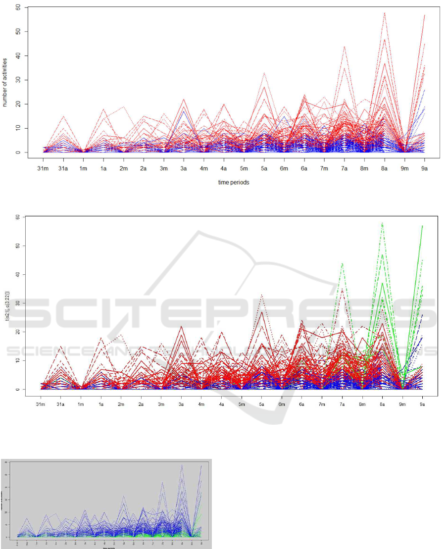
Figure 3: Plot showing activity of bees in two clusters given by kmeans.
Figure 4: Plot showing activity of bees in three clusters given by kmeans.
same result as Figure 3.
Figure 5: Plot showing activity of bees in two clusters given
by PAM.
Plotting the clusters means per hour of the two
clusters formed (see Figure 6), we can notice that one
cluster(red) shows an increasing mean activity respect
to days. Also, the highest activity is recorded between
the time interval from 2:00pm to 5:00pm. For the sec-
ond cluster (blue) the same trend is showed but bees
are less active.
4 FINDING THE TIME INTERVAL
WITH THE PEAK ACTIVITY
During the data wrangling process as well in the
clustering task, we noticed that most of bees’ ac-
tivity was between 8am and 8pm. Therefore,
first we did an analysis for four periods of time:
8:00am-11:00am, 11:00am-2:00pm, 2:00pm-5:00pm
and 5:00pm-8:00pm, We identified that the time-
period 2:00pm-5:00pm had the largest count of activ-
Clustering Honeybees by Its Daily Activity
603
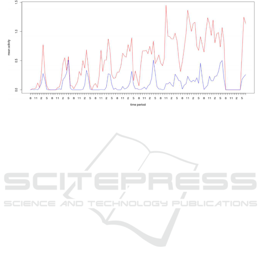
Figure 6: Plot showing means activity per hour of bees in the two clusters given by kmeans.
ity (1796) during the last four days, followed by the
time period 5:00pm-8:00pm. Finally, we carried out
an analysis by hour of the 380 bees during 8:00am-
8:00pm, and we found out that most of counting of
activity (809 counts) was from 2:00pm-3:00pm, fol-
lowed by the time period 1:00pm-2:00pm(582counts)
and in third place the time period 3:00pm-4:00pm
with 568 counts.
5 CONCLUSIONS
In this work, we have perform clustering on data
about bees’ daily activity during a time period of 10
days. According to the cluster validation measures we
decided to use two clusters as the optimum number.
Two categorial attrbutes ”Treatment” and ”Colony”
although were no used in the clustering process, they
are used in a posterior step to justyfy cluster for-
mation. Using a Chi-square test we conclude that
”treatment has no effect on the cluster formation, but
”Colony” and ”Treatment × Colony” affect indeed
the cluster formation.
Using data wrangling and visualization, we con-
clude that in one of the clusters the activity increases
with the time and remarkablly starting at the day
5. Furthermore, the highest bees’ activity occurs be-
tween 2:00pm to 3:00pm.
The R scripts and a R shiny program used in this
paper are available upon request from the first author.
ACKNOWLEDGEMENTS
This material is based upon work supported by
the National Science Foundation under Grant No.
1707355 and 1633184. BIGDATA:Collaborative Re-
search: Large-scale multi-parameter analysis of hon-
eybee behavior in their natural habitat.
REFERENCES
Bordier, C., Suchail, S., Pioz, M., Devaud, J., Colleta,
C., Charreton, M., Conte, Y. L., and Alaux, C.
(2017). Stress response in honeybees is associated
with changes in task-related physiology and energetic
metabolism. 98:47–54.
Grolemund, G. and Wickham, H. (2011). Dates and times
made easy with lubridate. 40(3):1–25.
Halkidi, M., Batistakis, Y., and Vazirgiannis, M. (2001). On
clustering validation techniques. 17:107–145.
Jain, A. and Dubes, R. (1988). Algorithms for clustering
data. Prentice-Hall, Inc., Upper Saddle River, NJ,
USA.
Prado, A., Pioz, M., Vidau, C., Requier, F., Jury, M.,
Crauser, D., Brunet, J.-L., Conte, Y. L., and Alaux, C.
(2019). Exposure to pollen-bound pesticide mixtures
induces longer-lived but less efficient honey bees.
650:1250–1260.
Robinson, G., Underwood, B., and Henderson, C. E.
(1984). A highly specialized water-collecting honey
bee. 15(3):355–358.
Tan, P., Steinbach, M., and Kumar, V. (2005). Introduction
to data mining. Addison-Wesley Longman Publishing
Co., Inc, Boston, MA, USA.
Tenczar, P., Lutz, C. C., Rao, V. D., Goldenfeld, N., and
Robinson, G. E. (2014). Automated monitoring re-
veals extreme interindividual variation and plasticity
in honeybee foraging activity levels. 95:41–48.
ICPRAM 2019 - 8th International Conference on Pattern Recognition Applications and Methods
604
