Constrained Multi Camera Calibration for Lane Merge Observation

Kai Cordes and Hellward Broszio

VISCODA GmbH, Hannover, Germany

Keywords:

Multi Camera Calibration, Lane Merge, Multi View, Vehicle Localization.

Abstract:

For the trajectory planning in autonomous driving, the accurate localization of the vehicles is required. Accu-

rate localizations of the ego-vehicle will be provided by the next generation of connected cars using 5G. Until

all cars participate in the network, un-connected cars have to be considered as well. These cars are localized

via static cameras positioned next to the road. To achieve high accuracy in the vehicle localization, the highly

accurate calibration of the cameras is required. Accurately measured landmarks as well as a priori know-

ledge about the camera conﬁguration are used to develop the proposed constrained multi camera calibration

technique. The reprojection error for all cameras is minimized using a differential evolution (DE) optimization

strategy. Evaluations on data recorded on a test track show that the proposed calibration technique provides

adequate calibration accuracy while the accuracies of reference implementations are insufﬁcient.

1 INTRODUCTION

Automated driving is regarded as the most promising

technology for improving road safety and efﬁciency

in the future (Fallgren et al., 2018). In the early phases

of partially automated driving, the driver is required to

constantly monitor the environment to be able to take

back the control of the vehicles whenever the need

arises. In the future, fully automated driving systems

will allow the driver to remain completely out of the

loop. Vehicles are expected to take over the complete

driving task.

1.1 Automated Driving, Cooperative

Maneuvers

As part of the automated driving tasks, a vehicle

should be able to perform appropriate maneuvers,

such as automatic lane changing whenever needed.

For this, the cooperation with nearby vehicles is cru-

cial. Cooperative maneuvers enhance the safety and

help the vehicles getting through difﬁcult trafﬁc si-

tuations. Vehicle-to-anything (V2X) communication

will ensure the distribution of information using a new

generation of mobile communication technology. A

major need is the accurate localization of the vehi-

cles (Fern

andez Barciela et al., 2017). The localiza-

tion of a vehicle is a main part of current research in

projects, such as 5GCAR

http://www.5gcar.eu

In addition to their self-localization capabilities,

vehicles are localized using external sensors, such as

cameras positioned nearby the road. This is crucial

for the integration phase, where only a subset of vehi-

cles is equipped with self-localizing and communica-

ting technology, the connected vehicles. The uncon-

nected vehicles are localized with a multi camera sy-

stem positioned near to the road. One important appli-

cation scenario for the joint localization of connected

and unconnected vehicles is the lane merge (Brahmi

et al., 2018).

1.2 Lane Merge Coordination

In the lane merge, one vehicle merges into a group

of vehicles driving on the motorway as shown in Fi-

gure 1. The goal is the coordination of driving trajec-

tories among a group of vehicles to improve the trafﬁc

safety and efﬁciency. A subject vehicle is coordina-

ted with remote vehicles driving on the main lane in

order to merge smoothly and safely into the lane wit-

hout collisions and with minimal impact on the traf-

ﬁc ﬂow. The trajectory recommendations are com-

puted based on road user properties such as position,

heading, and speed, continuously transmitted by the

connected cars. It is necessary that the system consi-

ders unconnected, i.e. non-communicating road users

as well. On the one hand, it cannot be assumed that

every road user is connected to the network. On the

other, remotely monitoring incorporates redundant or

even additional information to the system such as hig-

Cordes, K. and Broszio, H.

Constrained Multi Camera Calibration for Lane Merge Observation.

DOI: 10.5220/0007387805290536

In Proceedings of the 14th International Joint Conference on Computer Vision, Imaging and Computer Graphics Theory and Applications (VISIGRAPP 2019), pages 529-536

ISBN: 978-989-758-354-4

529

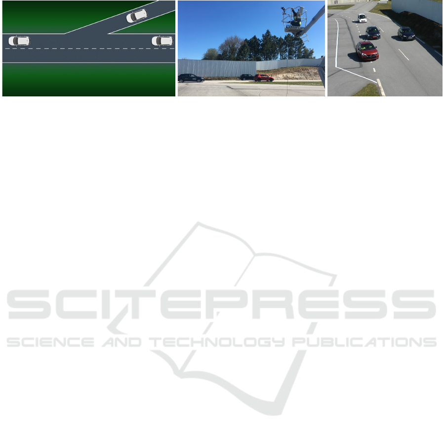
(a) Lane merge sketch (b) Video capture (c) Camera view

Figure 1: Sketch and video capture of the lane merge scenario using a mobile crane. One of the camera views while the lane

merge is performed is shown on the right.

her localization accuracy. This serves the goal of a

smooth lane merge without collisions and with mini-

mal impact on the trafﬁc ﬂow. For coordination and

vehicle feedback of trajectory recommendations and

the lane merge itself, a minimal viewing distance is

required, depending on the speed of the vehicles (Luo

et al., 2016). Thus, for the external observation of

the lane merge, more than one camera is needed. The

observation camera system is positioned next to the

road. The estimated vehicle data is sent to the lane

merge coordination entity via a cellular network. This

entity plans the cooperative maneuver and distribu-

tes corresponding instructions to connected vehicles,

while the behavior of unconnected vehicles is pre-

dicted and considered (Brahmi et al., 2018).

Since the positional accuracy is of key impor-

tance, a highly-accurate calibration is required. The

proposed approach incorporates geometric know-

ledge about the scene and about the installation of the

cameras. The scene knowledge consists of accurately

measured landmarks on the road. For the multi ca-

mera system, the height above the ground and relative

distances between the cameras are measured. This in-

formation in incorporated in a joint optimization of all

cameras.

1.3 Related Work

The accuracy demands for the camera calibration in

tracking applications depends on the tracking sce-

nario. While people trackers focus on the reliable

tracking in the 2D image plane (Milan et al., 2016;

Leal-Taix

e et al., 2017), vehicle tracking for coopera-

tive maneuvers requires highly accurate cameras for

two reasons: (1) tracking accuracy in 3D is of special

importance since collisions are to be avoided, and (2)

larger viewing distances are expected which increases

the demand for accurate 2D-3D correspondences.

In vehicle observation, most camera calibration

approaches make use of the road marking and assume

planar roads in the ﬁeld of view. Tang et al. (Tang

et al., 2018; Tang et al., 2017) use manually selected

lines on road markings for the calibration of the ca-

meras. The UA-DETRAC benchmark (Wen et al.,

2015) neglects camera calibration and focusses on 2D

detections with large variations regarding the vehi-

cle models, the recording conditions (different view-

points and weather conditions), and the vehicle den-

sity.

In contrast to these approaches, we focus on a very

speciﬁc setting, the lane merge. Since the goal is the

automated lane merge coordination, we observe one

car merging into the main lane of a multi-lane road

where several other cars are driving. One of the cars

on the main lane opens a gap for the incoming car.

The recorded data is expected to provide valuable in-

formation to learn trajectory recommendations for the

lane merge coordination entity. Since the setup requi-

res large viewing distances, accurate camera parame-

ters are required to fulﬁll the accuracy demand for the

localization of the vehicles.

We provide the following contributions:

• Practical solution for a suitable multi camera se-

tup dedicated to the lane merge observation sce-

nario

• Incorporation of easily measurable metrics of the

camera setup

• Evaluations with data recorded on a test track

show the accuracy improvements of the proposed

techniques.

In the following Section 2, the data recording se-

tup is brieﬂy described. In Section 3, the propo-

sed multi camera calibration approach is explained

in detail. Section 4 shows experimental results while

Section 5 concludes this paper.

2 LANE MERGE OBSERVATION

The data for the lane merge is recorded on a test track

which provides two lanes of approximately 100m

VISAPP 2019 - 14th International Conference on Computer Vision Theory and Applications

530

(a) CAM

(b) CAM

(d) CAM

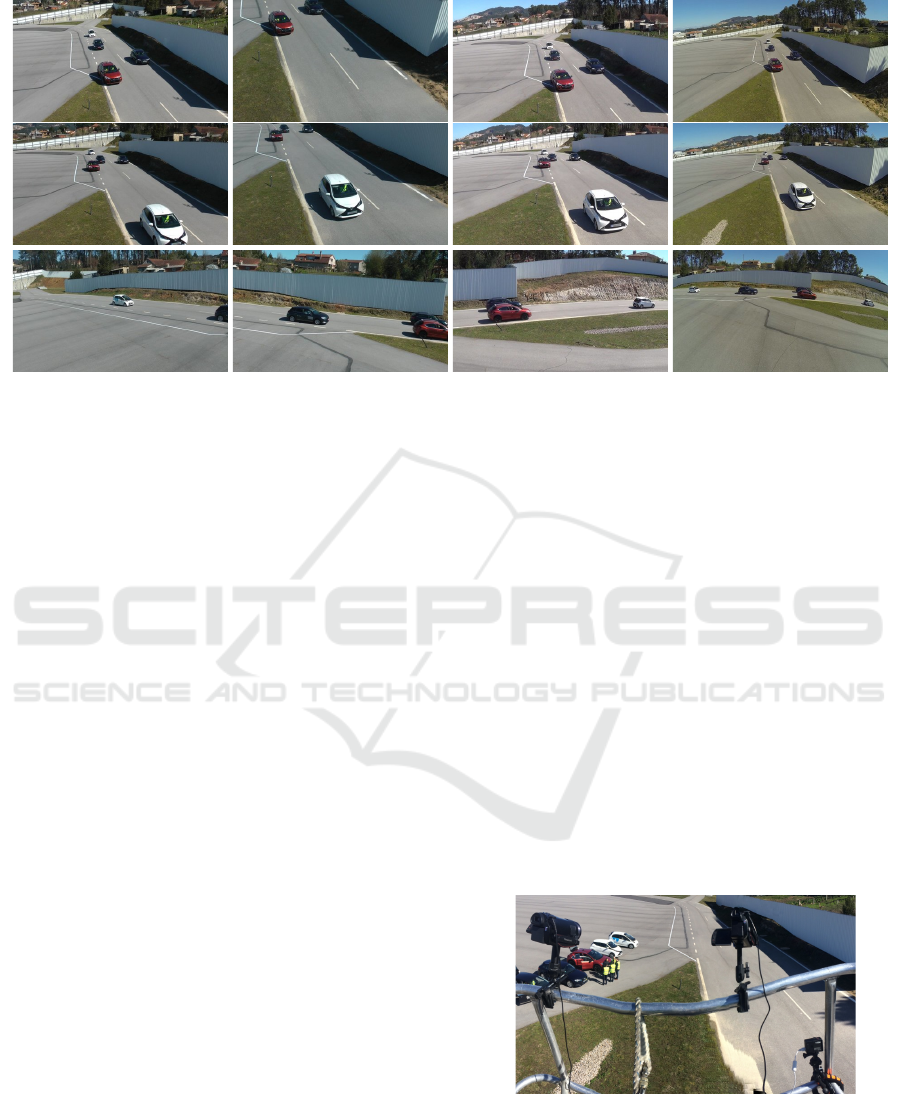
Figure 2: Video streams for the three sets (SET

(1)

, SET

(2)

, SET

(3)

from top to bottom). The temporal synchronization for

a set SET

(i)

is done manually. In one row, one point in time is shown for each set. The images demonstrate the lane merge

application. The camera calibration is done using landmarks as shown in Figure 4 using images without vehicles.

length for the main trafﬁc and the acceleration entry

lane for the merging car. The video capturing is done

with four video cameras attached to a mobile crane

(cf. Figure 1). The cameras capture 1920 × 1080

pixels at 50 fps. The temporal synchronization is done

manually in a post processing step using a video edi-

ting tool. For determining the synchronization, a pre-

viously deﬁned signal (headlight ﬂash) is recorded.

Using the manually determined signal in the video

sequences, all the video streams are synchronized as

shown in Figure 2. Four cars drive on the main lanes

while one car on the entry lane merges into the trafﬁc.

3 MULTI CAMERA

CALIBRATION

For the calibration, intrinsic and extrinsic camera pa-

rameters are required. For each camera, the radial dis-

tortion is computed in a preprocessing step using ma-

nually selected lines in the images (Thorm

ahlen et al.,

2003). For the computation of the extrinsic parame-

ters and the focal length (7 parameters), in contrast to

existing approaches in benchmark generation (Tang

et al., 2018; Tang et al., 2017), landmarks on the road

and their GPS positions are used. The GPS positi-

ons are determined using a D-GPS sensor with RTK

precision, which provides a localization accuracy of

approximately 2cm (RTK-DGPS: real time kinema-

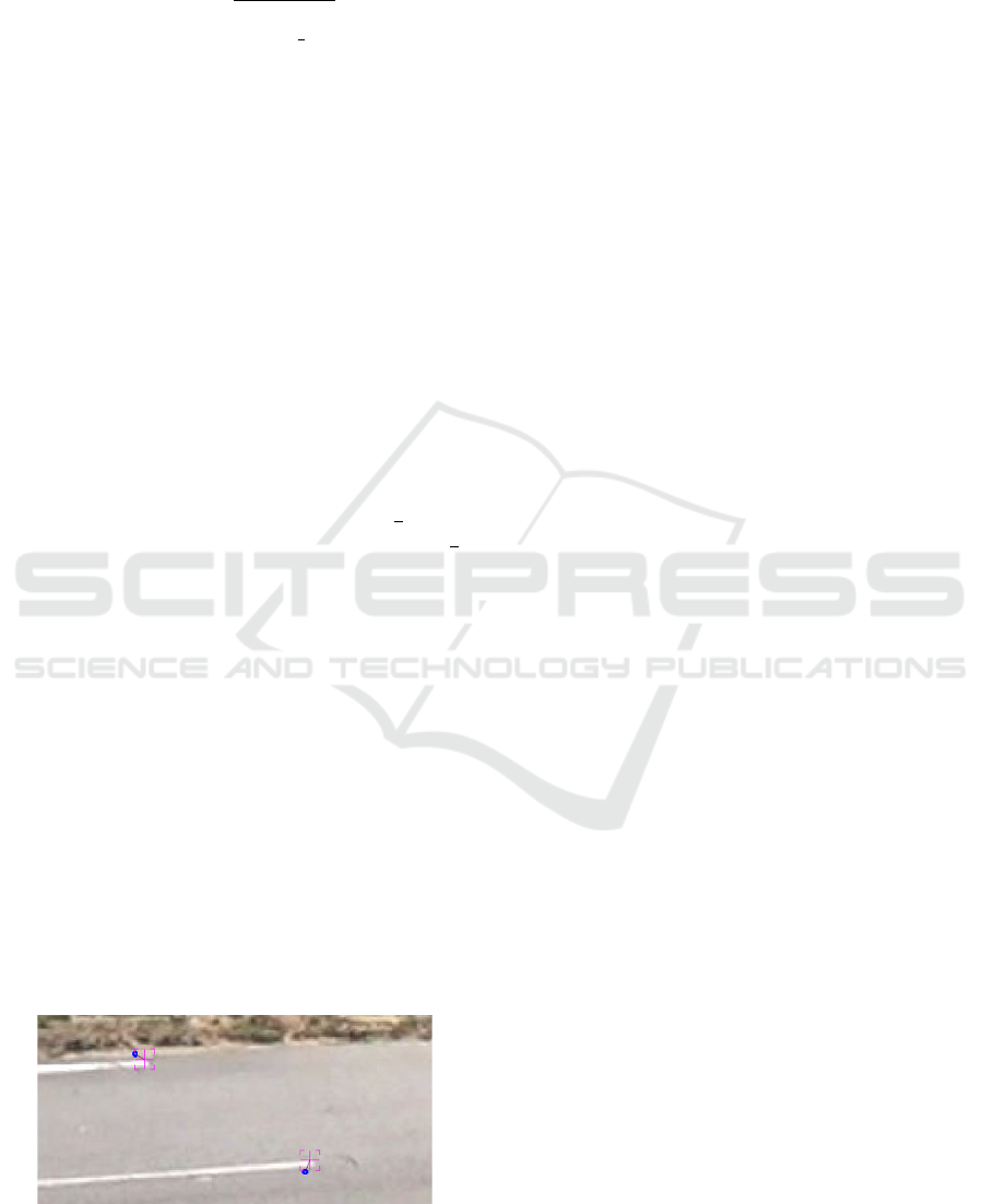
tics differential global positioning system). The land-

marks are selected such that (1) they are well distribu-

ted in the region of interest and (2) many of them are

visible in each camera view. Their positions are cho-

sen on edges of the road markings (ﬁfteen positions)

to ease the re-identiﬁcation in the camera images.

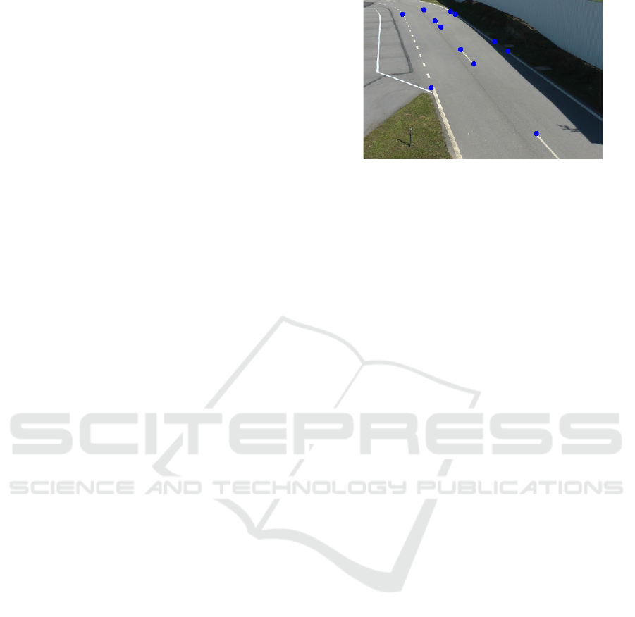
Additional geometrics of the camera setup are col-

lected using a laser scan tool which measures the

height of the camera (distance to the ground plane)

and relative distances between cameras. The camera

setup (example snapshot shown in Figure 3) is tested

for three different positions of the mobile crane with

differently mounted cameras to capture data sets with

different viewpoints.

The proposed calibration procedure leading to

accurate cameras is described in the following secti-

ons. It minimizes the reprojection error as deﬁned in

Section 3.1 uses an evolutionary optimizer shown in

Section 3.2, and is capable of incorporating a priori

known geometric constraints given in Section 3.3.

Figure 3: Panorama snapshot of three out of four cameras

from the observers perspective. The calibration technique

incorporates known distances between cameras. The dis-

tance between the top cameras is 77cm, the distance bet-

ween the top left and the bottom right camera is 127cm.

The basket size is 120 ×60cm, its height is 120cm.

Constrained Multi Camera Calibration for Lane Merge Observation

531

3.1 Cost Function

Using homogeneous coordinates, the 3D-2D corre-

spondence of object point P

∈ R

and feature point

j,k

∈ R

is given by the camera projection matrix

∈ R

3×4

j,k

= A

(1)

The standard technique for camera calibration is the

resectioning method (Tsai, 1987; Hartley and Zisser-

man, 2003), referred to as single camera optimization.

3.1.1 Single Camera Optimization

For optimizing each camera A

independently, the 3D

points P

with known 3D coordinates are projected

into the camera planes, resulting in 2D positions p

The known 2D representations

j,k

of the landmarks

are manually selected in the images. The squared dis-

tances d(

, A

)

determine the reprojection error:

∑

j=1

j,k

, A

)

(2)

The minimization of equation (2) with an appropriate

initialization for the camera matrix A

gives the cali-

bration result for each camera. A camera matrix is

built using the 7 parameters (C

, C

) (global coor-

dinate position) (pan, tilt, roll)-angles and the focal

length f (Hartley and Zisserman, 2003). The distance

(d(.))

is only computed if the 3D point is projected

into the visible region of the camera k resulting in dif-

ferent numbers of points J

for each camera.

3.1.2 Multi Camera Optimization

Multi camera calibration enables the joint optimiza-

tion of parameters, such as the knowledge that two ca-

meras have the same focal length. As shown in (Cor-

des et al., 2015), these additional costraints improve

the parameter estimation. The reprojection error is

then determined as:

ε =

∑

k=1

∑

j=1

j,k

, A

)

(3)

In our application, K = 4 cameras and up to

= 15 points are used, depending on the visibility

of the landmarks in each camera.

3.1.3 Constrained Multi Camera Optimization

Additional constraints for the calibration technique

are given by the camera setup, e.g. measured distan-

ces between two cameras or the height of a camera

above the ground plane. In each of our camera se-

tups, two cameras have nearly the same height above

Figure 4: Visualization of 12 of the 15 landmarks used for

the camera calibration.

the ground plane. Several of these constraints can be

easily exploited using spherical coordinates as shown

in Section 3.3. The global optimization for all para-

meters including special constraints measured in the

test scenario is done using evolutionary computation,

cf. Section 3.2.

3.2 Differential Evolution Optimization

For the minimization of the the cost function (3), the

Differential Evolution (DE) algorithm (Price et al.,

2005) is used. It is known as an efﬁcient global op-

timization method for continuous problem spaces. In

our application 4 cameras with 7 parameters each (po-

sition, orientation, focal length) are employed. The

number of estimated parameters determine the search

space dimension.

DE includes an adaptive range scaling for the ge-

neration of solution candidates. This enables global

search in the case where the solution candidate vec-

tors are spread in the search space and the mean dif-

ference vector is large. In the case of a converging

population the mean difference vector becomes smal-

ler. This enables efﬁcient ﬁne tuning towards the end

of the optimization process (Cordes et al., 2009).

For better convergence, the extended DERSF (DE

with Random Scale Factor) method proposed in (Das

et al., 2005) is used. It leads to a wider distribution

of the candidate vectors and, thus, improves the se-

arch. Since the dimension of the search space is high

(cf. Section 4.1), spreading the population helps in

achieving the global minimum of the cost function.

3.3 Incorporation of Geometric

Constraints

To limit the search space, additional constraints are

included in the optimization. This leads to faster con-

vergence and a higher probability of achieving the

global minimum of the cost function. Therefore, dis-

tances between cameras are provided. The incorpora-

VISAPP 2019 - 14th International Conference on Computer Vision Theory and Applications

532

tion is done using spherical coordinates. The mapping

from Euclidean coordinates to spherical coordinates

(x, y, z)

7→ (r, θ, φ)

, r ∈ R

, θ ∈ [0;π], φ ∈ [0;2π], is:













√

+ y

+ z

arccos(

)

arctan2(y, x)





(4)

The reverse mapping (r, θ, φ)

7→ (x, y, z)

is:













r · sin(θ) · cos(φ)

r · sin(θ) · sin(φ)

r · cos(θ)





(5)

We parameterize the ﬁrst camera position C

MAIN

in Euclidean coordinates and determine all other ca-

mera positions C

relative to the ﬁrst one with spheri-

cal coordinates. Then, r in equations (4) and (5) cor-

responds to the camera distance ||C

− C

MAIN

. For

example, the distance between the two top cameras

in Figure 3 is r = 77cm. Incorporating the relative

distances for each of the four cameras decreases the

number of estimated parameters by 3.

From equation (5), it follows that points with the

same height above the ground plane (and positive

orientation) lead to a relative angle θ of θ =

. Thus,

for the camera CAM

, the value θ can be set to θ =

because CAM

and CAM

are installed at the same

height h (cf. Figure 3). This decreases the number of

estimated parameters by 1.

Both options, the relative camera distance and set-

ting the same height of CAM

and CAM

, are explored

in Section 4 in experiments X

, X

, leading to the pro-

posed calibration technique. The incorporation of ge-

ometric constraints in the calibration greatly improves

its accuracy.

4 EXPERIMENTAL RESULTS

For the evaluation, three different camera sets SET

(1)

SET

(2)

, SET

(3)

are tested. Each set consists of four

cameras CAM

, . . . , CAM

attached to the basket of a

mobile crane as visualized in Figure 3. For SET

(1)

Figure 5: Example for the reprojection error (here ≈ 12 px

for both reprojected points shown in blue): The image de-

picts a small part of the calibration image of SET

(3)

, CAM

SET

(2)

the relative camera positions are approxima-

tely the same since only the crane basket height is

changed. The camera orientations were adjusted to

provide an appropriate ﬁeld of view for each camera.

For SET

(3)

, the mobile crane adopted a new position

and height. All cameras were removed and attached

to new positions at the basket of the crane. Images of

the cameras while the vehicles perform a lane merge

are shown in Figure 2. For the calibration, images

without vehicles are used as shown in Figure 4. The

images have a resolution of 1920 × 1080.

For all cameras, position, orientation, and focal

length are estimated. Since the cameras CAM

and

CAM

are identical, used with equal zoom factor, the

focal length of these cameras share the same estima-

tion value.

4.1 Setup

For the evaluation, four camera estimation experi-

ments X

, i = 1, . . . , 4 are deﬁned, two for single ca-

mera calibration and two for multi camera calibration.

The single camera calibration (X

, X

) is explained in

Section 3.1.1, the multi camera calibration (X

, X

) is

explained in Section 3.1.2. A priori known informa-

tion is incorporated as explained in Section 3.3.

: Estimation of all 7 parameters (position, orien-

tation, focal length) for each camera k indepen-

dently

: Estimation of 6 parameters - (C

, C

), orientation,

and focal length - with known ground truth height

= h

for each camera k independently

: Estimation of all parameters of the four cameras

using the information that (1) CAM

and CAM

have the same (unknown) height and (2) CAM

and CAM

have the same focal length (since these

cameras are identical), leading to 28 − 2 = 26 pa-

rameters

: Estimation like X

, additionally incorporating the

information of the relative distances r

between

CAM

and the other cameras, leading to 28 − 2 −

3 = 23 parameters

The relative camera distances r

and the camera

heights h

are measured after installation of the ca-

meras using a laser measure tool.

All approaches receive the same input data which

is the 3D positions of the 15 calibration markers and

their manually selected 2D positions in the images.

The radial distortion coefﬁcients are determined in a

preprocessing step.

The multi camera calibration approaches X

, X

get a very coarse initialization, such as viewing di-

rection towards the road and a square of 10m × 10m

Constrained Multi Camera Calibration for Lane Merge Observation

533

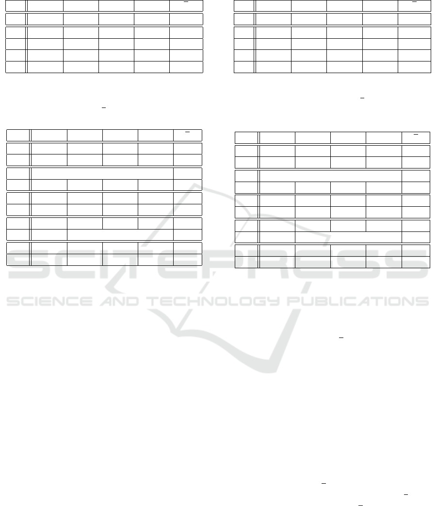
Table 1: Reprojection errors for single and the proposed

multi camera optimization for SET

(1)

. The distances are

measured in pel.

CAM

12 7 12 15

5.04 20.22 5.16 9.21 9.91

6.59 20.33 7.13 9.22 10.82

8.16 19.12 4.43 6.55 9.57

8.09 19.20 4.86 6.81 9.74

Table 2: Resulting camera heights h

and relative distances

for single and the proposed multi camera optimization for

SET

(1)

. Their mean error is e. The distances are measured

in m.

CAM

8.09 7.85 7.13 7.05 0.30

0.00 1.81 1.38 1.73 0.44

set to ground truth h

–

0.00 1.97 1.02 1.28 0.45

7.59 7.59 7.12 7.11 0.14

0.00 0.93 1.26 1.56 0.27

7.57 7.57 6.94 7.11 0.10

0.00 set to ground truth r

–

7.63 7.63 6.65 7.10 –

0.00 0.77 1.62 1.27 –

for the (C

, C

)-position while the single camera op-

timization techniques X

, X

, are fairly well initiali-

zed to achieve the best possible minimum of the cost

function. This is done with manual interaction. An

example for reprojected points

j,k

and their repro-

jection error is given in Figure 5.

Since the DE optimization used for X

, X

is based

on randomized generation of candidate vectors and a

random initialization (cf. Section 4.3), mean values

of 100 results are reported. The DE optimization em-

ploys common parameters (Price et al., 2005). The

number of particles is set to 300, the number of gene-

rations is 15000. The computation time is about 4 mi-

nutes on our I5 2.5 GHz notebook using unoptimized

code which is still appropriate for the calibration of

all cameras.

4.2 Accuracy Evaluation

The results are given for each of the three sets in-

dependently. We report the reprojection errors for

SET

(1)

, SET

(2)

, and SET

(3)

in Table 1, Table 3, and

Table 5, respectively. The comparisons with ground

truth measurements for the three sets are shown in

the Table 2, Table 4, and Table 6, respectively. The

heights h

of the cameras are determined with a la-

ser measure tool which provides high accuracy (er-

Table 3: Reprojection errors for single and the proposed

multi camera optimization for SET

(2)

. The distances are

measured in pel.

CAM

13 14 13 14

4.55 18.59 4.21 8.86 9.05

6.66 18.79 6.75 8.86 10.27

6.20 13.69 3.61 6.39 7.80

6.21 14.03 4.14 6.58 7.74

Table 4: Resulting camera heights h

and relative distances

for SET

(2)

. Their mean error is e. The distances are

measured in m. The relative camera distances r

are equal

to those in SET

(1)

CAM

5.76 5.27 4.77 4.90 0.21

0.00 1.12 1.37 1.62 0.32

set to ground truth h

–

0.00 0.98 0.96 1.29 0.30

5.39 5.39 4.77 4.89 0.10

0.00 1.04 1.03 1.41 0.24

5.45 5.45 4.65 4.83 0.08

0.00 set to ground truth r

–

5.42 5.42 4.44 4.89 –

0.00 0.77 1.62 1.27 –

ror ≈ 1mm), e.g. the height of the reference camera

CAM

for SET

(1)

is h

= 7.63m (ground truth), its

height for SET

(2)

is h

= 5.42m.

The experiments X

as reported in Section 4.1 lead

to reprojection errors ε

(cf. Tables 1, 3, and 5). For

simplicity, the mean errors ε are computed with the

same weight for each camera k, not regarding the

numbers of points J

. For the comparison with ground

truth measurements, the estimated camera heights h

and the relative camera distances r

are shown (cf. Ta-

bles 2, 4, and 6). These values are most demonstra-

tive to show the metrics and errors of the calibra-

tion results. Experiment X

lead to results for camera

height h

and relative camera distances r

. The entries

and r

at the bottom of each of the tables depict

the measured ground truth values for camera height

and relative distance.

In all evaluations SET

(1)

, SET

(2)

, and SET

(3)

, the

mean reprojection error ε tends to increase when more

constraints are added to the optimization, i.e. ε for ex-

periment X

is always larger than ε for experiment X

The same holds for experiment X

compared to expe-

riment X

(for SET

(2)

, the results are comparable).

But, the estimation for the relative distance r

experiment X

tend to better results for all three sets.

It follows that the reprojection error does not provide

VISAPP 2019 - 14th International Conference on Computer Vision Theory and Applications

534

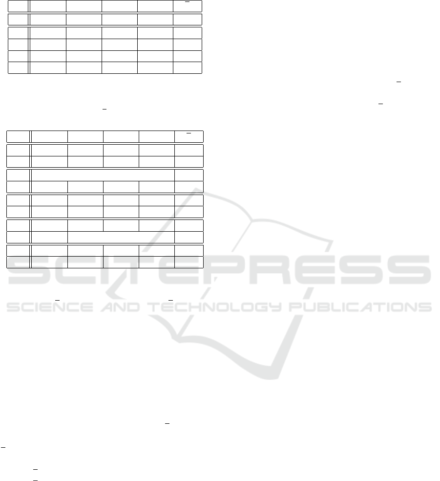
Table 5: Reprojection errors for single and the proposed

multi camera optimization for SET

(3)

. The distances are

measured in pel.

CAM

9 6 4 13

8.75 7.06 0.77 10.16 6.69

10.19 8.05 5.02 10.71 8.49

11.40 9.02 7.26 10.73 9.60

14.26 7.79 6.71 10.55 9.83

Table 6: Resulting camera heights h

and relative distances

for single and the proposed multi camera optimization for

SET

(3)

. Their mean error is e. The distances are measured

in m.

CAM

4.49 6.69 4.21 4.48 1.12

0.00 14.18 8.67 3.33 7.98

set to ground truth h

–

0.00 7.96 7.44 3.35 5.50

5.03 5.03 5.26 4.92 0.44

0.00 1.83 4.34 1.69 1.87

5.48 5.48 5.70 5.32 0.09

0.00 set to ground truth r

–

5.51 5.51 5.53 5.44 –

0.00 0.32 1.40 0.52 –

a good measure for the comparison of the accuracy.

Still, the results for r

are far from acceptable with a

mean error of e = 0.45m for SET

(1)

or even e = 5.50m

for SET

(3)

. To subsume, the error for the single ca-

mera calibration regarding camera height and relative

camera distance is surprisingly large. The reason is

the large uncertainty in the direction of the optical

axis of the camera. Variations of the camera posi-

tion in this direction does not affect the reprojection

error much. The small depth in the constellation of

the landmarks in SET

(3)

(side view of the road) make

this set the most challenging among these three.

The experimental setup X

improves the accuracy

results (r

, h

) signiﬁcantly, leading to e = 0.27m

for the mean relative camera distance for SET

(1)

and

e = 1.87m for SET

(3)

. The results for the estimated

camera height show acceptable values for SET

(1)

and

SET

(2)

(e = 0.14m and 0.10m), but large errors for

SET

(3)

(e = 0.44m). The mean relative camera dis-

tance error of 1.87m in SET

(3)

is still not acceptable.

The best results are achieved in experiment setup

leading to error distances of 0.10m, 0.08m, and

0.09m for the three camera sets. We can conclude

that X

provides the only usable solution for highly

accurate camera calibration.

4.3 Convergence Evaluation

To evaluate the robustness of the optimization, the

most challenging scenario SET

(3)

is examined. in Fi-

gure 6, we show mean and standard deviation of the

camera height for the experiments X

and X

The proposed method X

using the relative distan-

ces between the cameras (cf. Section 4.1 for details)

provides a stable and accurate solution while the ex-

periment X

comes to uncertain results. The mean

of the camera heights lead to an error of e = 0.44m

(cf. Table 6). The proposed approach using the expe-

rimental setup X

has a mean error of e = 0.09m.

5 CONCLUSIONS

For the targeted application of vehicle observation du-

ring a lane merge, a constrained multi camera calibra-

tion technique is designed. For the application, high

localization accuracy is required.

The proposed approach incorporates additional

constraints such as the relative distances between ca-

meras in the optimization. The distance measure-

ments can be done very easily during the camera in-

stallation. This makes the presented approach a very

useful part of the camera installation for the observa-

tion task.

The optimization procedure minimizes the repro-

jection error of known landmark positions on the

road. The global optimization is based on evolutio-

nary computation and provides suitable convergence

behaviour on all test sets. For the accuracy evaluation,

the resulting camera heights are compared. The pro-

posed approach provides a mean error in the camera

height below 10cm for cameras installed at a height

of 5.4-7.6m observing landmarks with a distance of

up to 100m.

ACKNOWLEDGEMENTS

This work has been performed in the framework of

the H2020 5GCAR project co-funded by the EU. The

authors would like to acknowledge the contributions

of their colleagues from 5GCAR.

Constrained Multi Camera Calibration for Lane Merge Observation

535

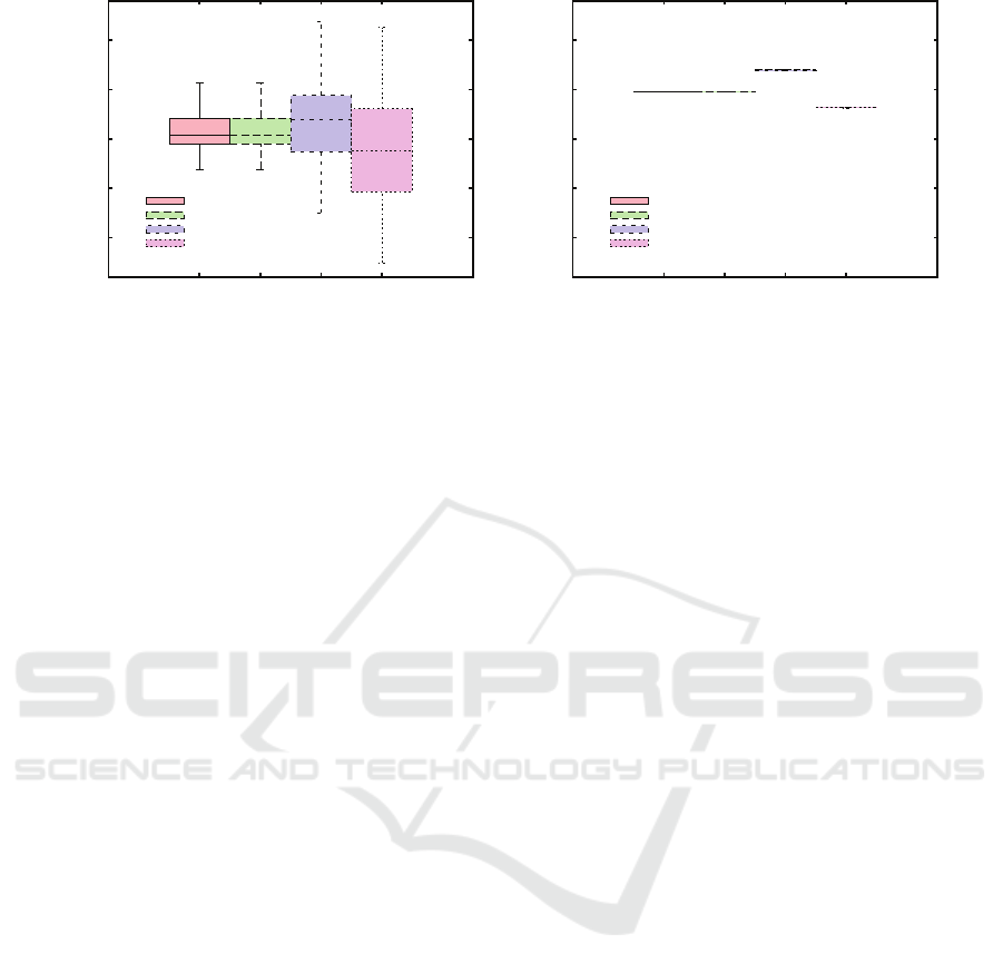
4.5

5.5

1 2 3 4

height [m]

CAM1

CAM2

CAM3

CAM4

(a) Experiment X

: camera heights of SET

(3)

4.5

5.5

1 2 3 4

height [m]

CAM1

CAM2

CAM3

CAM4

(b) Experiment X

: camera heights of SET

(3)

Figure 6: Mean and standard deviation for 100 evaluations of the camera height for experiments X

(a) and X

(b)

(cf. Section 4.1). Here, the most challenging SET

(3)

is shown. For X

, much smaller standard deviations are achieved.

REFERENCES

Brahmi, N., Frye, T., Marti

nan, D., Dafonte, P., Abad,

X., S

aez, M., Cellarius, B., Gangakhedkar, S., Cao,

H., Sequeira, L., Berger, K., Theillaud, R., Otter-

bach, J., Grudnitsky, A., Villeforceix, B., Allio, S.,

Lefebvre, M., Odinot, J.-M., Tiphene, J., Servel, A.,

Fern

andez Barciela, A. E., Broszio, H., Cordes, K.,

and Abbas, T. (2018). 5GCAR Demonstration guide-

lines. https://5gcar.eu/. [Online; accessed 20-October-

2018].

Cordes, K., Hockner, M., Ackermann, H., Rosenhahn, B.,

and Ostermann, J. (2015). WM-SBA: Weighted multi-

body sparse bundle adjustment. In IAPR International

Conference on Machine Vision Applications (MVA),

pages 162–165.

Cordes, K., Mikulastik, P., Vais, A., and Ostermann, J.

(2009). Extrinsic calibration of a stereo camera sy-

stem using a 3D CAD model considering the uncer-

tainties of estimated feature points. In European Con-

ference on Visual Media Production (CVMP) , pages

135–143.

Das, S., Konar, A., and Chakraborty, U. K. (2005). Two im-

proved differential evolution schemes for faster global

search. In Annual Conference on Genetic and Evo-

lutionary Computation, GECCO 05, pages 991–998.

ACM.

Fallgren, M., Dillinger, M., Li, Z., Vivier, G., Abbas, T.,

Alonso-Zarate, J., Mahmoodi, T., Alli, S., Svensson,

T., and Fodor, G. (2018). On selected V2X technology

components and enablers from the 5GCAR project. In

IEEE International Symposium on Broadband Multi-

media Systems and Broadcasting (BMSB), pages 1–5.

Fern

andez Barciela, A. E., Servel, A., Tiphene, J., Fallgren,

M., Sun, W., Brahmi, N., Str

om, E., Svensson, T.,

Bernardez, D., Zarate, J. A., Kousaridas, A., Boban,

M., Dillinger, M., Condoluci, M., Mahmoodi, T., Li,

Z., Otterbach, J., Lefebvre, M., Vivier, G., Abbas, T.,

and Wing

ard, P. (2017). 5GCAR scenarios, use ca-

ses, requirements and KPIs. https://5gcar.eu/. [Online;

accessed 20-October-2018].

Hartley, R. I. and Zisserman, A. (2003). Multiple View Ge-

ometry. Cambridge University Press, second edition.

Leal-Taix

e, L., Milan, A., Schindler, K., Cremers, D., Reid,

I. D., and Roth, S. (2017). Tracking the trackers:

An analysis of the state of the art in multiple object

tracking. arXiv:1704.02781.

Luo, Y., Xiang, Y., Cao, K., and Li, K. (2016). A dynamic

automated lane change maneuver based on vehicle-

to-vehicle communication. Transportation Research

Part C: Emerging Technologies, 62:87–102.

Milan, A., Leal-Taix

e, L., Reid, I. D., Roth, S., and Schind-

ler, K. (2016). MOT16: A benchmark for multi-object

tracking. arXiv:1603.00831.

Price, K. V., Storn, R., and Lampinen, J. A. (2005). Dif-

ferential Evolution - A Practical Approach to Global

Optimization. Natural Computing Series. Springer,

Berlin, Germany.

Tang, Z., Wang, G., Liu, T., Lee, Y., Jahn, A., Liu, X., He,

X., and Hwang, J. (2017). Multiple-kernel based vehi-

cle tracking using 3D deformable model and camera

self-calibration. arXiv:1708.06831.

Tang, Z., Wang, G., Xiao, H., Zheng, A., and Hwang, J.-

N. (2018). Single-camera and inter-camera vehicle

tracking and 3D speed estimation based on fusion of

visual and semantic features. In IEEE Conference on

Computer Vision and Pattern Recognition Workshop

(CVPRw), pages 108–115.

Thorm

ahlen, T., Broszio, H., and Wassermann, I. (2003).

Robust line-based calibration of lens distortion from a

single view. Proceedings of Mirage, pages 105–112.

Tsai, R. (1987). A versatile camera calibration technique

for high-accuracy 3D machine vision metrology using

off-the-shelf tv cameras and lenses. IEEE Journal on

Robotics and Automation, 3(4):323–344.

Wen, L., Du, D., Cai, Z., Lei, Z., Chang, M., Qi, H., Lim,

J., Yang, M., and Lyu, S. (2015). UA-DETRAC:

A new benchmark and protocol for multi-object de-

tection and tracking.

arXiv:1511.04136

VISAPP 2019 - 14th International Conference on Computer Vision Theory and Applications

536