
Risk Analysis of Distributed Generation Scenarios
Paula Medina Maçaira, Margarete Afonso de Sousa, Reinaldo Castro Souza
and
Fernando Luiz Cyrino Oliveira
Industrial Engineering Department, Pontifícia Universidade Católica do Rio de Janeiro,
Rua Marquês de São Vicente, 225, Rio de Janeiro, Brazil
Keywords: Forecasting, Time Series, Hydroelectric Power Generation, Distributed Generation, Small Hydropower
Plant, Exogeneous Variables.
Abstract: Assertiveness in generation forecast is an important issue for utilities when they are planning their
operation. Hydropower Generation forecast has a strong stochastic component and thinking about small
hydropower plants (SHP) is even more complex. In recent years, many SHP was installed in Brazil due to a
Government incentive and the distributed generation penetration has an impact in technical losses’
estimation. The objective of this study is to propose a methodology to generate synthetic scenarios of
distributed generation for hydro sources. A case study was carried on with historical generation data from
SHP located in Minas Gerais. The periodic regression model was considered the best model for forecast
hydropower generation. Three distributed generation scenarios are obtained using Conditional Value at Risk
analysis after combining multiple scenarios from inflow forecasting generated with the periodic regression
model.
1 INTRODUCTION
The Brazilian electricity generation system, called as
National Interconnected System (NIS), is mainly
composed by hydroelectric plants. In December
2017, the installed power capacity was
approximately 155 GW and hydroelectric generation
represented 67.8% of this total. To complement the
electricity matrix there are also thermal, wind power
and other kinds of source (ONSa, 2018).
According to the Brazilian legislation,
hydroelectric plants that generate between 5 and 30
MW, with a reservoir area that not exceeds 13 km
2
,
are called Small Hydroelectric Power Plants (SHP).
There is also Reduced Capacity Generating Plants
(RCGP) that produces 5 MW or less and do not have
reservoirs. This type of plants has low
environmental impact and represents 3.7% of NIS
installed capacity nowadays (ABRAPCH, 2018).
In order to encourage the alternative energy
sources, like SHP, wind and biomass, the Brazilian
Government created a program called PROINFA.
Such program increases the numbers of SHP and
RCGP, reaching nowadays 436 and 683,
respectively, in operation in Brazil (ANEEL, 2018;
ABRAPCH, 2018).
Hydroelectric generation depends on the amount
of water in the rivers that depends mostly on
precipitation. The rainfall can vary within an hour, a
month, a year and, also, between the years. And this
alternation between dry and wet periods affects the
amount of power generation (Maçaira et al., 2017;
Lima et al., 2014).
Given this, the future generation from hydro
sources must be estimated considering its past
generation and also considering exogenous
information, such as inflows and precipitation.
The estimation of technical losses is also an
important issue for utilities. To do so, they have to
forecast future generation. For hydro sources with
strong stochastic components, improve generation
forecats is fundamental to achieve better results.
In many situations, for SHP and RCGP, there are
no inflows data available. Therefore, the main
objective of this study is to use inflow time series
from neighboring basins as exogenous variables
(Lohmann et al., 2016), via Linear Regression
models, in order to predict SHP and RCGP future
generation. To build future scenarios it is proposed a
methodology based on historical power generation
and CVaR risk analysis. With this approach the
utilities could provide better forecast power
378
Maçaira, P., Afonso de Sousa, M., Souza, R. and Oliveira, F.
Risk Analysis of Distributed Generation Scenarios.
DOI: 10.5220/0007389203780383
In Proceedings of the 8th International Conference on Operations Research and Enterprise Systems (ICORES 2019), pages 378-383
ISBN: 978-989-758-352-0
Copyright
c
2019 by SCITEPRESS – Science and Technology Publications, Lda. All rights reserved

generation and, consequentely, aid in the prediction
of technical losses, due to the distributed generation
penetration. A case study was carried out to test the
methodology accuracy.
This paper is organized in 4 sections. Section 1 is
the introduction and presents the motivation of this
paper. Section 2 presents an explanation of the
metodology used. The discussions and results are
presented in section 3 and in section 4 the
conclusion of this study and its final considerations
are shown.
2 METHODOLOGY
Time series models are popular and useful for long-
term forecasting and simulation. There is a wide
variety of methods that meet this purpose and the
choice of a suitable one for modeling a particular
problem depends on many factors, such as: amount
of time series available, precision required, period of
time available, the ability to interpret results, among
others.
Among time series univariate methods, the most
popular belongs to the Box & Jenkins family (Box
and Jenkins, 1976; Box et al., 1994). These models
consider only time series historical and according to
Salas et al., (1982) natural phenomena are, in
general, stationary.
In this field, the most applied models are
periodic ones. They have the ability to capture the
dependence not only of the time interval between
observations, but also of the data period (Moss and
Bryson, 1974). The most used are the Periodic
Autoregressive (PAR) and the Periodic
Autoregressive Moving Average (PARMA).
With the Computer Science advances, methods
that incorporate external information to improve
time series forecasting and/or simulation have
gained space. Recent studies confirm the
applicability forecasting models using external
information. It means that appropriate use of
exogenous variables makes the prediction models
more robust with ample possibility to represent
future events with different characteristics from
those that happened in the past.
In a recent study, Maçaira et al., (2018) show
that, in Environmental Sciences area, such kind of
models have produced better results. The most used
are: Linear Regression, Artificial Neural N,
ARIMAX and Support Vector Machine.
In this study, the candidate models used for
forecast the generation time series are Regression
Linear ones.
Considering a time series , with periods (
12 for monthly time series), the number of years
and is number of steps-aheads. So,
,
,
,
,…,
,
,…,
,
. As the time series,
in this study, have a seasonal/periodic component,
the first model tested is a Seasonal Average. It
means that the forecast for any given month will
always be the historical average for that month, as
Equation 1.
,
,
(1)
The second model proposed, named as Seasonal
Naïve, forecasts, for any given month, the last
historical observation of those month, as shown in
Equation 2.
,
,
(2)
In the same way as the first model, these two
methodologies are considered as benchmarks.
However, among the models proposed, the
Seasonal Autoregressive Integrated Moving Average
– SARIMA
,,
,,
is a traditional
one. This is a univariate model for stationary and
non-stationary series (Box and Jenkins, 1976; Box et
al., 1994).
The next two proposed models are Linear
Regression ones. It means that the exogenous
variable, inflow series, that explains power
generation behavior (Hyndman and Athanasopoulos,
2013).
In the first linear regression model, as shown in
Equation 3, there is no consideration of seasonality
represented by the months within the year. Unique
(intercept) and
(slope) are obtained from the
data.
,
,
(3)
The second linear regression model takes into
account the periodic monthly effect. In this case, 12
coefficients
(intercept) and 12 coefficients
(slope) are estimated, one for each month.
,
,
,
,
(4)
To compare all these models, two metrics have been
used. The Root Mean Square Error (RMSE) and the
Mean Absolute Percentage Error (MAPE).
∑
(5)
Risk Analysis of Distributed Generation Scenarios
379

100
1
(6)
Where
is the time series value in period ,
is the
adjusted value on period and is the total of
observations.
After the best model has been chosen, the next
step consists of simulate synthetic scenarios for
power generation. According to the Brazilian
legislation, for small hydropower plants, the object
of this study, power generation is considered as
“distributed generation”.
Hence, to generate these artificial time series, it
will be combined synthetic scenarios from the
independent variable and the model selected. In this
case study, the data is from hydro sources, so the
independent variable are the inflows time series. To
to so, the methodology is the same used by the
official model in Brazil, which combines Periodic
Autoregressive model (PARp) with LogNormal
distributed probability. For more details, see
Oliveira et al., (2015) and Charbeneau (1978).
If the Periodic Regression model is chosen
(equation 4), the distributed generation scenarios are
obtained as shown in Equation 7, where
1,…, and is the number of scenarios generated.
,
,
,
,
,,
(7)
By this methodology it is possible to obtain a great
number of scenarios that implies in choosing which
are the ones of interest. According to the literature,
to do so, risk measures, as Value at Risk (VaR) and
Conditional Value at Risk (CVaR) are used.
VaR is the maximum potential loss (or worst
loss) valuation at a specified confidence interval (
confidence level) that an investor would be exposed
within a considered time horizon. The VaR can be
translated as the amount in which the losses do not
exceed 1% of the scenarios. The VaR
calculation is quite simple, since it is, by definition,
some quantile associated with a distribution extreme
percentile (usually 1% or 5%). For example, it can
calculate the worst result among the best 95% or the
best among the worst 5%. This cut off value is 5%
VaR. A criticism related to VaR is that it does not
provide the expected loss size estimation since the
loss has exceeded the critical value, that is, it does
not bring any information about the losses greater
than the value found for the quantile1
(Rockafellar and Uryasev, 2002).
CVaR is a measure that indicates the average
loss that exceeds VaR, it means, it quantifies "how
big" is the average loss (risk) exposure. CVaR is
considered a coherent measure of risk (Artzner et
al., 1999) and is more pessimistic than VaR. It is
used to measure losses. Therefore, while the VaR
answers the question "What is the minimum loss
incurred by the portfolio in% worst scenarios?",
The CVaR answers the question "What is the
average loss incurred by the portfolio in % worst
scenarios?". A great benefit of using CVaR over
VaR is in detecting the maximum acceptable losses.
The software R is used, in this study to fit all
models and to present results (R Core Team,2015).
3 RESULTS AND DISCUSSIONS
The power plant Ivan Botelho II SHP is in operation
since November 28, 2003, with installed capacity of
12.4 MW. It is located in Minas Gerais and will be
used as a case study to test the methodology
accuracy.
For the proposed approaches, the inflow monthly
data base of Ivan Botelho II SHP is required. The
historical power generation was provided by the
company who owns the SHP concession, but the
inflow data with an enough historical size to allow
the realization of this study was not available. This
way, was used neighbouring inflows data provided
by the National Electric System Operator (ONSb,
2018). To find the highest correlation (temporal and
spatial) with power generation, 32 Hydroelectric
Power Plants (HPP) inflow data, located in Rio de
Janeiro, Minas Gerais and Espírito Santo, were
analysed.
The Sobragi power plant, located at Paraibuna
River, in Minas Gerais, was the one that presented
the highest correlation with Ivan Botelho II SHP.
Figure 1 shows the both power generation and
inflow between January 2010 and December 2016.
Although the start date of Ivan Botelho II is January
2004, the inflow data of Sobragi available is from
January 2010 and to use regression models the two
series may have the same length.
Figure 1: Sobragi HPP inflow and Ivan Botelho II SHP
power generation.
ICORES 2019 - 8th International Conference on Operations Research and Enterprise Systems
380
In order to check the predictive power of each
proposed methodology, the generation series was
split into training period (Jan/2010 to Dec/2016) and
validation (Jan/2017 to Dec/2017). Table 1 shows
the results for in-sample and out-of-sample
adjustment with the RMSE and MAPE error metrics.
The behavior for each approach is shown in Figure
2.
Table 1: RMSE and MAPE comparative results.
Model
In-sample Out-of-sample
MAPE
(%)
RMSE
(MWh)
MAPE
(%)
RMSE
(MWh)
Periodic
Regression
15,96 827,74 33,24 685,22
SARIMA 18,53 1040,40 45,97 1841,55
Linear
Regression
21,57 1135,43 29,41 809,72
Seasonal
Average
25,09 1651,45 52,03 2328,09
Naive
Seasonal
33,13 1567,34 35,23 1347,13
Figure 2: 12-step-ahead out-of-sample Ivan Botelho II
SHP forecasts.
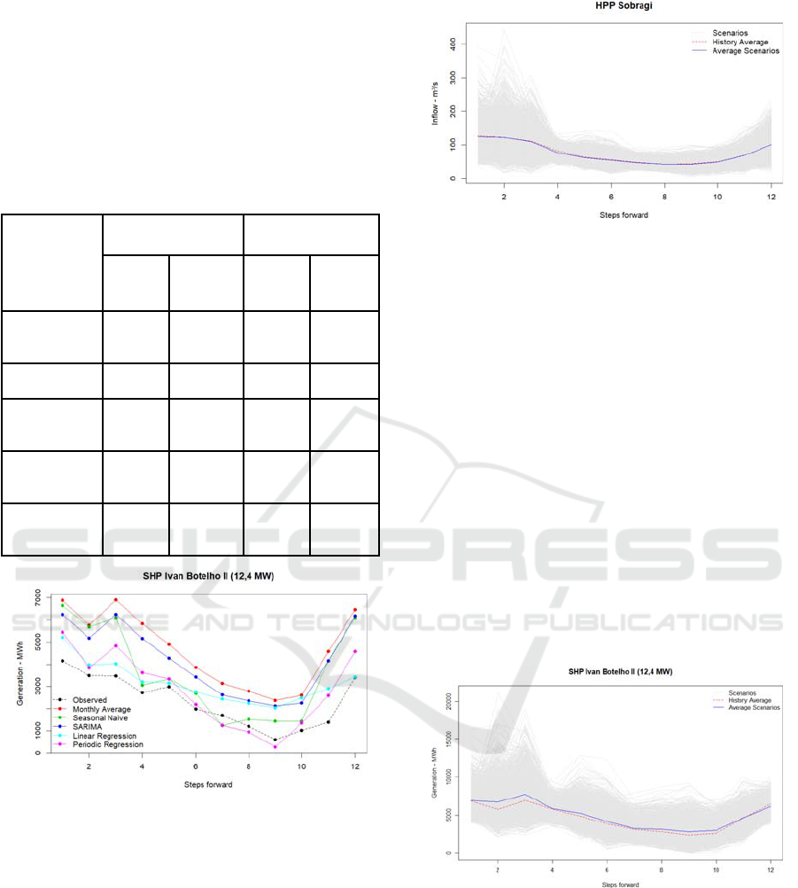
Therefore, 2,000 synthetic scenarios for Sobragi
inflow data, with 12-step-ahead out-of-sample
forecast,
were simulated via PARp model and
LogNormal probability distribution, as explained in
the Methodology section. The scenarios, historical
average observed and Sobragi inflow average
scenarios are presented in Figure 3.
Figure 3: Sobragi HPP inflow synthetic scenarios.
By combining the estimated model through
Periodic Regression (Equation 8) and the inflow
scenarios (Figure 3), it was possible to obtain 2,000
distributed generation scenarios for Ivan Botelho II,
as shown in Figure 4.
,
,
0.2850.806
,,
,
,
0.1351.041
,,
,
,
0.1621.317
,,
,
,
0.0921.498
,,
,
,
0.0652.171
,,
,
,
0.1122.182
,,
,
,
0.1792.382
,,
,
,
0.2002.673
,,
,
,
0.2172.588
,,
,
,
0.1011.820
,,
,
,
0.0251.473
,,
,
,
0.3540.669
,
,
(8)
Figure 4: Ivan Botelho II SHP distributed generation
synthetic scenarios.
Considering the assumption that the greatest risk
of technical losses occurs when the distributed
generation penetration is greater, the selection of
interest scenarios occurred through the CVaR
with1%,5%,10%. The extracted scenarios are
shown in Figure 5.
Risk Analysis of Distributed Generation Scenarios
381
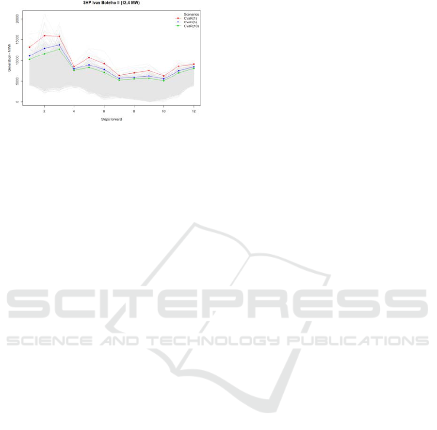
Figure 5: Scenarios obtained by CVaR risk measure with
1%,5%,10%.
4 FINAL CONSIDERATIONS
The main objective of this paper is to provide energy
generation scenarios for the further estimation of
technical losses. Hydro sources are strongly
dependent on hydrological regimes, and because of
this, the power generation forecast models from such
sources should consider exogenous variables such as
inflow and/or precipitation in order to obtain more
robust and accurate forecasts. The case of study is
from a SHP plant located in Brazil that has no
hydrological data available. So the first methodology
developed seeks neighboring hydrological series that
explain the small plants generation series. This
approach involves the test of many techniques in
order to find the most suitable forecast model. With
the purpose of build energy generation scenarios it
was used the periodic autoregressive model, from
Box & Jenkins, and the Conditional Value at Risk
analysis.
The proposed methodology to find the most
correlated basin inflow with the SHP generation
present good results and as consequence the periodic
regression that uses the inflow database as
exogenous variable was the method that shows the
smallest error metrics (RMSE and MAPE). The
CVaR 1%, 5% and 10% have been shown to be
efficient to select scenarios that can provide highest
technical losses since when more energy is
generated from SHP greater are the technical losses.
For further studies, it is possible to apply this
methodology with other types of distributed
generation, as wind power. It is also possible, to
continue the research, to execute the complete cycle,
it means with the scenarios obtained, simulate the
technical losses and compare with real data.
Another research path could be the use of
dummies variables to explain low generation, in
several times due to maintenance periods.
ACKNOWLEDGEMENTS
This study was financed in part by the Coordenação
de Aperfeiçoamento de Pessoal de Nível Superior -
Brasil (CAPES) - Finance Code 001. The authors
also thank the R&D program of the Brazilian
Electricity Regulatory Agency (ANEEL) for the
financial support (P&D 06585-1802/2018) and the
support of the National Council of Technological
and Scientific Development (CNPq - 304843/2016-
4) and FAPERJ (202.673/2018).
REFERENCES
ABRAPCH. 2018. O que são PCHs e CGHs. Associação
Brasileira de Pequenas Centrais Hidrelétricas e
Centrais Geradoras Hidrelétricas. Avaiable at
http://www.abrapch.org.br/pchs/o-que-sao-pchs-e-
cghs (accessed date June 15, 2018).
Artzner, P., Delbaen, F., Eber, J. M., Heath, D., 1999.
Coherent measures of risk. Mathematical Finance, vol.
9, no. 3.
BRASIL. ANEEL, 2015. Resolução Normativa nº 673, de
4 de Agosto de 2015. Estabelece os requisites e
procedimentos para obtenção de outorga de
autorização para exploração de aproveitamento de
potencial hidráulico com características de Pequena
Central Hidrelétrica – PCH, Available at
http://www2.aneel.gov.br/cedoc/ren2015673.pdf
[accessed date October 5, 2018].
Box, G. E. P., Jenkins, G. M., 1976. Time Series Analysis:
Forecasting and Control. Holden-Day, San Francisco,.
Box, G. E. P., Jenkins, G. M., Reinsel, G. C., 1994. Time
Series Analysis: Forecasting and Control. Prentice
Hall.
Charbeneau, R. J., 1978. Comparison of the two and three-
parameter log normal distributions used in streamflow
synthesis. Water Resource Research, 1978,14(1):149–
50.
Hyndman, R., Athanasopoulos, G. 2013. Forecasting:
principles and practice. Avaiable at http://
otexts.com/fpp/ (accessed date July 7, 2018).
Lima, L. M. M., Popova, E., Damien, P., 2014. Modeling
and forecasting of Brazilian reservoir inflows via
dynamic linear models. International Journal of
Forecasting, 30(3):464–476.
Lohmann, T., Hering, A. S.,Rebennack, S., 2016. Spatio-
temporal hydro forecasting of multireservoir inflows
for hydro-thermal scheduling. European Journal of
Operational Research, 255(1):243–258.
Maçaira, P. M., Cyrino Oliveira, F. L., Ferreira, P. G. C.,
Almeida, F. V. N., Souza, R. C., 2017. Introducing a
causal PAR(p) model to evaluate the influence of
climate variables in reservoir inflows: a Brazilian
case. Pesquisa Operacional (Impresso), v. 37, p. 107-
128.
ICORES 2019 - 8th International Conference on Operations Research and Enterprise Systems
382

Maçaira, P. M., Thomé, A. M. T., Cyrino Oliveira, F. L.,
Ferrer, A. L. C., 2018. Time series analysis with
explanatory variables: A systematic literature review.
Environmental Modelling & Software, vol. 107, pag.
199-209.
Moss, M. E., Bryson, M. C., 1974. Autocorrelation
structure of monthly streamflows. Water Resources
Research, vol. 10, pag. 737-744.
Oliveira, F. L. C., Souza, R.C., Marcato, A. L. M., 2015. A
time series model for building scenarios trees applied
to stochastic optimisation. International Journal of
Electrical Power & Energy Systems, v. 67, p. 315-323.
ONS, 2018a. Operador Nacional do Sistema Elétrico.
Avaiable at http://ons.org.br/paginas/sobre-o-sin/o-
que-e-o-sin (accessed date June 25 ,2018).
ONS. 2018b. Resultados da Operação – Histórico da
Operação - Dados Hidrológicos/Vazões. Avaiable at
http://ons.org.br/Paginas/resultados-da-
operacao/historico-da-
operacao/dados_hidrologicos_vazoes.aspx [accessed
date July 10, 2018].
Rockafellar, R. T., Uryasev, S., 2002. Conditional value-
at-risk for general loss distributions. Journal of
Banking & Finance, vol. 26, no. 7.
Salas, J. D., Boes, D. C., Smith, R. A., 1982. Estimation of
ARMA Models with seasonal parameters. Water
Resources Research, vol. 18, no. 4, pag. 1006-1010.
R Core Team. 2015. The R Project for Statistical
Computing. Avaiable at https://www.r-project.org/
[accessed date March 20, 2018].
Risk Analysis of Distributed Generation Scenarios
383
