Extracting Vehicle Sensor Signals from CAN Logs for Driver

Re-identiﬁcation

Szilvia Lesty

, Gergely Acs

, Gergely Bicz

and Zsolt Szalay

CrySyS Lab, Dept. of Networked Systems and Services, Budapest Univ. of Technology and Economics, Hungary

Dept. of Automotive Technology, Budapest Univ. of Technology and Economics, Hungary

Keywords:

Driver Re-identiﬁcation, CAN Bus, Sensor Signals, Privacy, Reverse Engineering, Machine Learning, Time

Series Data.

Abstract:

Data is the new oil for the car industry. Cars generate data about how they are used and who’s behind the wheel

which gives rise to a novel way of proﬁling individuals. Several prior works have successfully demonstrated

the feasibility of driver re-identiﬁcation using the in-vehicle network data captured on the vehicle’s CAN

(Controller Area Network) bus. However, all of them used signals (e.g., velocity, brake pedal or accelerator

position) that have already been extracted from the CAN log which is itself not a straightforward process.

Indeed, car manufacturers intentionally do not reveal the exact signal location within CAN logs. Nevertheless,

we show that signals can be efﬁciently extracted from CAN logs using machine learning techniques. We

exploit that signals have several distinguishing statistical features which can be learnt and effectively used

to identify them across different vehicles, that is, to quasi ”reverse-engineer” the CAN protocol. We also

demonstrate that the extracted signals can be successfully used to re-identify individuals in a dataset of 33

drivers. Therefore, not revealing signal locations in CAN logs per se does not prevent them to be regarded as

personal data of drivers.

1 INTRODUCTION

Our digital footprint is growing at an unprecedented

scale. We use numerous devices and online services

creating massive amount of data 24/7. Some of these

data are personal, either concerning an identiﬁed or

and identiﬁable natural person; thus, they fall under

the protection of the European General Data Protec-

tion Regulation (GDPR) (European Union, 2016b).

In fact, to determine whether a natural person is iden-

tiﬁable based on given data, one should take account

of all means reasonably likely to be used (by the data

controller or an adversary) to identify the natural per-

son. Such a technique is, e.g., singling out; whether

it is reasonably likely to be used depends on the spe-

ciﬁc data and the scoio-technological context it was

collected in (European Union, 2016a).

One speciﬁc area where digitalization and data

generation are booming is automotive. From a set

of mechanical and electrical components, cars have

evolved into smart cyber-physical systems. Whereas

this evolution has enabled automakers to implement

advanced safety and entertainment functionalities, it

has also opened up novel attack surfaces for malicious

hackers and data collection opportunities for OEMs

and third parties. The backbone of a smart car is

the in-vehicle network which connects ECUs (Elec-

tronic Control Units); the most established vehicu-

lar network standard is called Control Area Network

(CAN) (Voss, 2008). CAN is already a critical tech-

nology worldwide making automotive data access a

commodity. One or more CAN buses carry all impor-

tant driving related information inside a car. OEMs

(Original Equipment Manufacturers, i.e., car makers)

collect and analyze CAN data for maintenance pur-

poses; however, CAN data might reveal other, more

personal traits, such as the driving behavior of natu-

ral persons. Such information could be invaluable to

third party service providers such as insurance com-

panies, ﬂeet management services and other location-

based businesses (not to mention malicious entities),

hence there exist economic incentives for them to col-

lect or buy them.

It has been shown that automobile driver ﬁnger-

printing could be practical based on sensor signals

captured on the CAN bus in restricted environments

(Enev et al., 2016). Using machine learning tech-

niques, authors re-identiﬁed drivers from a ﬁxed set

136

Lestyán, S., Acs, G., Biczók, G. and Szalay, Z.

Extracting Vehicle Sensor Signals from CAN Logs for Driver Re-identiﬁcation.

DOI: 10.5220/0007389501360145

In Proceedings of the 5th International Conference on Information Systems Security and Privacy (ICISSP 2019), pages 136-145

ISBN: 978-989-758-359-9

of experiment participants, thus implementing sin-

gling out, which makes this a privacy threat. There

is a caveat: the adversary has to know the higher

layer protocols of CAN in order to extract meaning-

ful sensor readings. Since such message and mes-

sage ﬂow speciﬁcations (above the data link layer) are

usually proprietary and closely guarded industrial se-

crets, such adversarial background knowledge might

not be reasonable. In this case, the research question

changes: is it possible for an adversary to re-identify

drivers based on raw CAN data without the knowl-

edge of protocols above the data link layer?

Contributions. In this paper we investigate experi-

mentally the potential to identify and extract vehicle

sensor signals from raw CAN bus data for the sake of

inferring personal driving behavior and re-identifying

drivers. As signal positions, lengths and coding are

proprietary and vary among makes, models, model

years and even geographical area, ﬁrst, we have to

interpret the messages. We emphasize that we do not

intend to perform (an even remotely) comprehensive

reverse engineering (Sija et al., 2018); we focus solely

on a small number of sensor signals which are good

descriptors of natural driving behavior.

Our contributions are three-fold:

1. we devise a heuristic method for message decom-

position and log pre-processing;

2. we build, train and validate a machine learning

classiﬁer that can efﬁciently match vehicle sensor

signals to a ground truth based on raw CAN data.

In particular, we train a classiﬁer on the statistical

features of a signal in one car (e.g., Opel Astra),

then we use this trained classiﬁer to localize the

same signal in a different car (e.g., Toyota). The

intuition is that the physical phenomenon repre-

sented by the signal has identical statistical fea-

tures across different cars, and hence can be used

to identify the same signal in all cars using the

same classiﬁer;

3. we brieﬂy demonstrate that re-identiﬁcation of

drivers is possible using the extracted signals.

The rest of the paper is structured as follows. Sec-

tion 2 presents related work. Section 3 gives a back-

ground on important characteristics of the Controller

Area Network. Section 4 describes our data collec-

tion process. Section 5 presents our efforts on mes-

sage decomposition and log pre-processing. Section

6 presents the design, evaluation and validation of

our random forest classiﬁer for extracting sensor sig-

nals. Section 6.4.2 brieﬂy demonstrates the success-

ful application of the extracted signals for driver re-

identiﬁcation. Finally, Section 7 concludes the paper.

2 RELATED WORK

Driver characterization based on CAN data has gath-

ered signiﬁcant research interest from both the au-

tomotive and the data privacy domain. The com-

mon trait in these works is the presumed familiarity

with the whole speciﬁc CAN protocol stack including

the presentation and application layers giving the re-

searchers access to sensor signals. This knowledge is

usually gained via access to the OEM’s documenta-

tions in the framework of some research cooperation.

As such, researchers do not normally disclose such

information to preserve secrecy.

Miyajima et al. has investigated (Miyajima et al.,

2007) driver characteristics when following another

vehicle and pedal operation patterns were modeled

using speech recognition methods. Sensor signals

were collected in both a driving simulator and a real

vehicle. Using car-following patterns and spectral

features of pedal operation signals authors achieved

an identiﬁcation rate of 89.6% for the simulator (12

drivers). For the ﬁeld test, by only applying cep-

stral analysis on pedal signals the identiﬁcation rate

was down to 76.8% (276 drivers). Fugiglando et

al. (Fugiglando et al., 2018) developed a new method-

ology for near-real-time classiﬁcation of driver be-

havior in uncontrolled environments, where 64 peo-

ple drove 10 cars for a total of over 2000 driving

trips without any type of predetermined driving in-

struction. Despite their advance use of unsupervised

machine learning techniques they conclude that clus-

tering drivers based on their behavior remains a chal-

lenging problem.

Hallac et al. (Hallac et al., 2016) discovered

that driving maneuvers during turning exhibit per-

sonal traits that are promising regarding driver re-

identiﬁcation. Using the same dataset from Audi and

its afﬁliates, Fugiglando et al. (Fugiglando et al.,

2017), showed that four behavioral traits, namely

braking, turning, speeding and fuel efﬁciency could

characterize driver adequately well. They provided a

(mostly theoretical) methodology to reduce the vast

CAN dataset along these lines.

Enev et al. authored a seminal paper (Enev et al.,

2016) which makes use of mostly statistical features

as an input for binary (one-vs-one) classiﬁcation with

regard to driving behavior. Driving the same car in a

constrained parking lot setting and a longer but ﬁxed

route, authors re-identiﬁed their 15 drivers with 100%

accuracy. Authors had access to all available sensor

signals and their scaling and offset parameters from

the manufacturer’s documentation.

In a paper targeted at anomaly detection in in-

vehicle networks (Markovitz and Wool, 2017), au-

Extracting Vehicle Sensor Signals from CAN Logs for Driver Re-identiﬁcation

137

thors developed a greedy algorithm to split the mes-

sages into ﬁelds and to classify the ﬁelds into cat-

egories: constant, multi-value and counter/sensor.

Note that the algorithm does not distinguish between

counters and sensor signals, and the semantics of the

signals are not interpreted. Thus, their results cannot

be directly used for inferring driver behavior.

3 CAN: CONTROLLER AREA

NETWORK

The Controller Area Network (CAN) is a bus system

providing in-vehicle communications for ECUs and

other devices. The ﬁrst CAN bus protocol was devel-

oped in 1986, and it was adopted as an international

standard in 1993 (ISO 11898). A recent car can have

anywhere from 5 up to 100 ECUs, which are served

by several CANs. Our point of focus is the CAN serv-

ing the drive-train.

CAN is an overloaded term (Szalay et al., 2015).

Originally, CAN refers to the ISO standard 11898-

1 specifying the physical and data link layers of the

CAN protocol stack. Second, another meaning is

connected to FMS-CAN (Fleet Management System

CAN), originally initiated by major truck manufactur-

ers, deﬁned in the SAE standard family J1939; FMS-

CAN gives a full-stack speciﬁcation including recom-

mendations on higher protocol layers. Third, CAN

refers to the multitude of proprietary CAN protocols

which are make and model speciﬁc. This results in

different message IDs, signal transformation parame-

ters and encoding. These protocols are usually based

on the standardized lower layers, but their higher lay-

ers are kept conﬁdential by OEMs. The overwhelm-

ing majority of cars use one or more proprietary CAN

protocols. Generally, sensor signals in CAN variants

have a sampling frequency in the order of 10 ms.

On the other hand, using the standard on-board di-

agnostics (OBD, OBD-II) is a popular way of getting

data out of the car. Originally developed for mainte-

nance and technical inspection purposes and included

in every new car since 1996, OBD is also used for

telematics applications. Adding to the confusion re-

garding CAN, OBD has ﬁve minor variations includ-

ing one which is based on the CAN physical layer.

Sensor signals carried by OBD have a sampling fre-

quency in the order of 1 second. In certain vehicle

makes and models, one or more CANs are also con-

nected to the OBD2-II diagnostic port. In such cars,

also utilizing OBD over the CAN physical layer, it

is possible to extract ﬁne-grained CAN data via an

OBD-II logger device.

Table 1 shows a simpliﬁed picture of a CAN mes-

sage with a 11-bit identiﬁer, which is the usual format

for everyday cars; trucks and buses usually use the ex-

tended 29-bit version. This example shows an already

stripped message, i.e., we do not discuss end of frame

or check bits.

Components of a CAN Bus Message.

• Timestamp: Unix timestamp of the message

• CAN-ID: contains the message identiﬁer - lower

values have higher priority (e.g. wheel angle,

speed, ...)

• Remote Transmission Request: allows ECUs to

request messages from other ECUs

• Length: length of the Data ﬁeld in bytes (0 to 8

bytes)

• Data: contains the actual data values in hexadeci-

mal format. The Data ﬁeld needs to be broken to

sensor signals, transformed and/or converted to a

human-readable format in order to enable further

analysis.

Throughout this paper, we focus on the three prac-

tically relevant ﬁelds: CAN-ID, Length and Data.

4 DATA COLLECTION

As CAN data logs are not widely available, we con-

ducted a measurement campaign. For data collection

in particular we connected a logging device to the

OBD-II port and logged all observed messages from

various ECUs. Such a device acts as a node on the

CAN bus and is able to read and store all broadcasted

messages. Our team developed both the logging de-

vice (based on a Raspberry PI 3) and the logging soft-

ware (in C). Note that it is common that the OBD2

connector is found under the steering wheel. Also

note that not all car makes and models connect the

CAN serving the drive-train ECUs (or any CAN) to

the OBD-II port (e.g., Volkswagen, BMW, etc.); in

this case we could not log any meaningful data.

We have gathered meaningful data from 8 differ-

ent cars and a total number of 33 drivers. We did not

put any restriction on the demographics of the dif-

ferent drivers or the route taken. In each case we

asked the driver to drive for a period of 30-60 min-

utes, while our device logged data from every route

the drivers took. Drivers were free to choose their

way, but still conforming to three practical require-

ments: (1) record at least 2 hours of driving in total,

(2) do not record data when driving up and down on

hills or mountains, (3) do not record data in extremely

heavy trafﬁc (short runs and idling). Free driving was

recorded for all 33 drivers with an Opel Astra 2018:

ICISSP 2019 - 5th International Conference on Information Systems Security and Privacy

138

Table 1: Example of CAN messages.

Timestamp CAN-ID Request Length Data

1481492683.285052 0x0208 000 0x8 0x00 0x00 0x32 0x00 0x0e 0x32 0xfe 0x3c

1497323915.123844 0x018e 000 0x8 0x03 0x03 0x00 0x00 0x00 0x00 0x07 0x3f

1497323915.112910 0x00f1 000 0x6 0x28 0x00 0x00 0x40 0x00 0x00

13 people were between the age of 20-30, 12 between

30-40, and 8 above 40; there were 5 women and 28

men; 11 with less experience (less than 7000 km per

year on average or novice driver), 9 with average ex-

perience (8-14000 km per year), and 13 with above

average experience (more than 14000 km per year).

We gathered data from the following cars: Citroen

C4 2005 (22 message IDs), Toyota Corolla 2008 (36

IDs), Toyota Aygo 2014 (48 IDs), Renault Megane

2007 (20 IDs), Opel Astra 2018 (72 IDs), Opel As-

tra 2006 (18 IDs), Nissan X-trail 2008 (automatic, 34

IDs) and Nissan Qashqai 2015 (60 IDs). We would

like to emphasize that the two Opel Astras use com-

pletely different prorpietary CAN versions (even the

only 2 common IDs correspond to completely dif-

ferent Data). We also recorded the GPS coordinates

via an Android smartphone during at least one logged

drive per car. Most routes were driven inside or close

to Budapest; approximately 15-20% was recorded on

a motorway.

5 CAN DATA ANALYSIS

All recorded messages contained 4 to 8 bytes of data;

this made it likely that multiple (potentially unrelated)

pieces of information can be sent under the same

ID. We ﬁrst assumed that signals are positioned over

whole bytes; this turned out to be wrong. Our in-

vestigation revealed that besides signal values a mes-

sage can also contain constants, multi-value ﬁelds and

counters. Some values appear only on-demand, such

as windscreen or window signals. All data apart from

sensor signals are considered noise and, therefore,

need to be removed.

Meaningful CAN IDs vary signiﬁcantly across ve-

hicle makes and models, therefore we expected that

the only signals found in all cars with high probability

are the basic ones: such as velocity, brake, clutch and

accelerator pedal positions, RPM (round per minute)

and steering wheel angle. Next, we devise a method

that yields a deeper understanding of the Data ﬁeld

in CAN messages and a possibility for sensor signal

extraction. Note that from this point we will use the

term ID as a reference to both a given type of message

and its data stream (time series).

5.1 Bit Decomposition Heuristics

Extracting the signals from a CAN message is not a

trivial challenge. While monitoring the data stream

while driving and ﬁnding the exact bits that change in

reaction to one’s actions is possible, it is highly time

consuming, does not scale with hundreds of different

existing CAN protocol versions and bound to miss

out on potential sensor signals. (We only took this

approach with a single car model to generate train-

ing data and a validation framework for our machine

learning solution.) Our objective here is to present our

observations on message types and distributions that

leads to a smarter message decomposition method.

First, we examined the message streams literally

bit-by-bit. We presumed that inside a given ID with

potentially multiple sensor readings there was a dif-

ference in their bit value distribution, hence they

could be systematically located and partitioned ac-

cording to some rule. E.g., let us assume that there

are two signals sent next to each other under the same

ID (i.e., there are no zero bits or other separators be-

tween the two. Given that signals are encoded in a

big endian (little endian) format, both of their MSBs

(LSBs) are rarely 1s. Therefore, there should be a

drop in bit probability (i.e., the probability for a given

bit to be 1) between the last bit of the ﬁrst signal and

the ﬁrst bit of the second signal. In order to visualize

these drops we represent IDs by their bit distribution:

we sum the number of messages for each ID and how

many times a given bit was one and divide these two

measures:

∑

|v|

j=1

=1}

|v|

where v denotes the binary vector of a given ID,

that is the representation of a CAN message’s payload

in binary format, and where v

denotes the probability

of a bit being 1 at the i

position.

When we examined the distribution of the bits in

an ID we found that that in some cases it is straight-

forward to extract a signal: between two signal candi-

dates there were separator bits with v

= 0 or v

= 1.

Other cases were more complex: given Figure 1(a)

it is hard to determine signal borders. However,

combined with the bit distribution from the same ID

and car model but another drive, the signals became

clearly distinguishable.

Extracting Vehicle Sensor Signals from CAN Logs for Driver Re-identiﬁcation

139

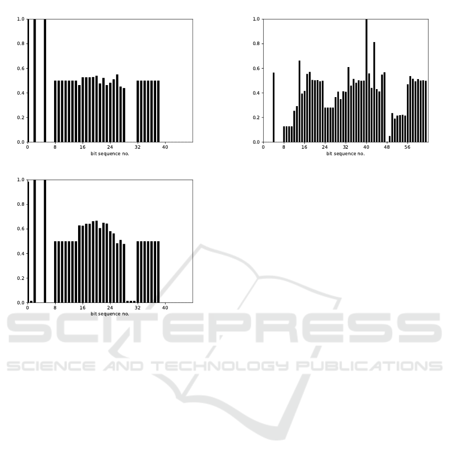
(a) Driver A

(b) Driver B

Figure 1: Bit distribution of the same ID from different

drivers.

5.2 Pre-processing

After examining bit distributions we realized that ≈

90% of candidate signal blocks are placed on one or

two bytes. In other cases signal borders were not un-

ambiguous, see Figure 2. Our ﬁrst heuristic suggests

a start of a new signal because of the drop at the 23rd

and the 24th bits, although it is clearly a counter or

a constant on 3 bits, but we can not determine where

exactly a new signal starts (is it the 28th bit or the

32nd?). Moreover, the 41th bit is constant 1 bit which

might signify some kind of a separator, yet we cannot

be certain. After a long evaluation we decided to di-

vide the data part of the messages to bytes and pairs

of bytes; as a result for one ID we could deﬁne 4 to 8

sensor candidates.

Filtering. Examining the byte time series resulting

from the above approach, we spotted that many se-

ries were constant, had very few values, were cyclic

(counters) or changed very rarely. As we intended

to use machine learning to ﬁnd the exact signals, not

ﬁltering these samples could have caused signiﬁcant

performance loss and a bloated and skewed training

dataset with a lot of similar negative samples resulting

Figure 2: Consecutive blocks in a CAN message that cannot

be unambiguously divided.

in a decreased variability of training data potentially

to a degree of corrupting the model. Therefore, we

evaluated the variation for each sample and excluded

those that had a very low variation (”low variation”

was also a free variable optimized during evaluation).

Normalization. We scaled all candidate time series

to the interval of [0, 1]: we extracted the maximum

value for the whole candidate series, then we divided

all values by the maximum. Scaling the data solves

the problem of transformed (shifted) values, i.e., the

same signal can take different values during drives,

that can be a result of some transformation on the

data in one vehicle or simply the fact that one car was

driven in a lower range of velocity in contrast to the

other (i.e., one log comes from a drive that did not ex-

ceed 50 km/h while the other rarely drove slower than

100 km/h).

Sliding Windows. We divided logs into overlap-

ping sliding windows from which we extracted our

features for machine learning. The sliding window

length (elapsed time) and percentage of overlap with

previous and successive windows were free variables

which we set to default values and subsequently opti-

mized during run time.

6 CLASSIFICATION

We use machine learning for two purposes; ﬁrst, to

extract signals from CAN messages, and second, to

perform driver re-identiﬁcation using the extracted

signals. Therefore, we build two different types of

classiﬁers. In order to extract signals, we train a clas-

siﬁer per signal on the statistical features of the signal

in a base car (e.g., Opel Astra 2018) where we ex-

actly know where the signal resides, that is, the mes-

sage ID and byte number of the CAN message which

contains the signal. Then, we use the trained models

to identify the same signals in another car (e.g., Toy-

ICISSP 2019 - 5th International Conference on Information Systems Security and Privacy

140

ota) where the locations of the signals (i.e., message

ID and byte number) are unknown. The intuition is

that the physical phenomenon that a signal represents

has identical statistical features irrespective of the car,

and hence can be used to identify the same signal in

all cars using the same classiﬁer.

For driver re-identiﬁcation, similarly to previous

works (Fugiglando et al., 2018; Miyajima et al.,

2007), we use a separate classiﬁer that is trained on

the already extracted signals of the car. This classiﬁer

learns the distinguishing features of different drivers

(and not that of signals like the ﬁrst classiﬁer) using

the signals produced during their drives.

For both signal extraction and driver re-

identiﬁcation, the features computed from each

sliding window constitute a single training sample

(i.e., a sample vector) used as the input of our

machine learning classiﬁers. Below we describe

the classiﬁers, the division of training and test-

ing samples, and the method used for multi-class

classiﬁcation.

6.1 Multi-class Classiﬁcation

We implemented multiclass classiﬁcation using bi-

nary classiﬁcation in a one-vs-rest way (aka, one-vs-

all (OvA), one-against-all (OAA)). The strategy in-

volves training a single classiﬁer per class, with the

samples of that class as positive samples and all other

samples as negatives. For signal extraction, a class

represents a pair of message ID and byte number,

whereas for driver re-identiﬁcation, it represents a

driver’s identity. A random forest model was trained

per class with balanced training data (i.e., containing

the same number of positive and negative samples),

and its output was binary indicating whether the input

sample belongs to the class or not. For signal extrac-

tion, as each training/testing sample is a small portion

of the time-series (i.e., window) representing a signal,

we apply the trained model on all portions of a signal

and obtain multiple decisions per signal. Then, the

”votes” are aggregated and the candidate signal with

the most number of ”votes” is selected.

We would like to stress that random forests are in-

deed capable of general multiclass classiﬁcation with-

out its transformation to binary. We have also tried

this general multiclassiﬁcation approach, however, its

results were inferior to the OvA’s results. More-

over successful driver re-identiﬁcation can already

be carried out using a single or only a few signals

(Enev et al., 2016). In this paper, we use the veloc-

ity, the brake pedal, the accelerator pedal, the clutch

pedal and the RPM signals to extract for driver re-

identiﬁcation.

Table 2: Average feature importances.

Feature Importance

count below mean 0.2113

count above mean 0.1482

cid ce 0.1290

mean abs change 0.1048

maximum 0.0716

longest strike below mean 0.0708

6.2 Feature Extraction

Our classiﬁers use statistical features of the samples;

for each sliding window we extracted 20 different

statistics that are widely considered as most descrip-

tive regarding time series characteristics (see the best

features in Table 2. We ﬁnally used 15 features based

on their importances calculated from our random for-

est models. These features are the following:

1. count above mean(x): Returns the number of val-

ues in x that are higher than the mean of x.

2. count below mean(x): Returns the number of

values in x that are lower than the mean of x.

3. longest strike above mean(x): Returns the

length of the longest consecutive subsequence in

x that is bigger than the mean of x.

4. longest strike below mean(x): Returns the

length of the longest consecutive subsequence in

x that is smaller than the mean of x.

5. binned entropy(x, max bins): First bins the val-

ues of x into max bins equidistant bins. The

max bin parameter was generally set to 10. Then

calculates the value of:

−

∑

min(max bins,len(x))

k=0

· log(p

) · 1

>0}

where p

is the percentage of samples in bin k.

6. mean abs change(x): Returns the mean over the

absolute differences between subsequent time se-

ries values which is:

∑

i=1,...,n−1

i+1

− x

7. mean change(x): Returns the mean over the dif-

ferences between subsequent time series values

which is:

∑

i=1,...,n−1

i+1

− x

)

8. OTHER: minimum, maximum, mean, median,

standard variation, variance, kurtosis, skewness

This way we created an input vector of features for

each sample (one sample corresponds to one win-

dow). No smoothing, outlier elimination or function

approximation are performed on the samples before

Extracting Vehicle Sensor Signals from CAN Logs for Driver Re-identiﬁcation

141

feature extraction. For calculating the above statis-

tics, we used the ts f resh python package

6.3 Training and Model Optimization

For training our classiﬁer we need to have a ground

truth of sensor signals from a single car. These cer-

tiﬁed signals then can be compared to the candidate

signals from other cars to ﬁnd the best match. We

chose the Opel Astra 2018 as our reference, as we

had the most drives logged from this car.

Velocity versus GPS. We recorded GPS coordinates

for all drives with the Opel Astra 2018. Setting the

Android GPS Logger app to the highest accuracy

(complemented by cell tower information achieving

an accuracy of 3 meters) and saving the coordinates

every second, we ended up with a time series of lo-

cations. Using the timestamps, GPS time series also

determines the mean velocity between neighboring

locations, producing a velocity time series. Intu-

itively, the GPS based velocity is very close to the one

recorded from the CAN bus.

In order to test this hypothesis we applied the Dy-

namic Time Warp algorithm (DTW) (Salvador and

Chan, 2007). The DTW algorithm is part of time se-

ries classiﬁcation algorithms (Bagnall et al., 2016),

their important characteristic being that there may be

discriminatory features dependent on the ordering of

the time series values (Geurts, 2001). A distance mea-

surement between time series is needed to determine

similarity between time series and for classiﬁcation.

Euclidean distance is an efﬁcient distance measure-

ment that can be used. The Euclidean distance be-

tween two time series is simply the sum of the squared

distances from each n

point in one time series to the

point in the other. The main disadvantage of us-

ing Euclidean distance for time series data is that its

results are very un-intuitive. If two time series are

identical, but one is shifted slightly along the time

axis, then Euclidean distance may consider them to

be very different from each other. DTW was intro-

duced to overcome this limitation and give intuitive

distance measurements between time series by ignor-

ing both global and local shifts in the time dimension.

DTW ﬁnds the optimal alignment between two time

series if one time series may be warped non-linearly

by stretching or shrinking it along its time axis.

Before running DTW we excluded the outliers

from the GPS-based velocity series. These points are

the result of GPS measurement error and materialize

in extreme differences between two neighboring ve-

locity values (we used 30 km/h as a limit). We then

ran DTW with the GPS-based velocity values against

https://tsfresh.readthedocs.io/en/latest/

Table 3: DTW velocity search top results.

CAN ID Byte Distance

0410 1-2 7499

0410 2-3 15972

0295 1-2 20609

0510 2 20981

0510 3 21585

all other sensor candidates of the CAN log. As the re-

sult of the DTW algorithm is a distance between two

series, the smallest distance yields the best match: in

every case it was indeed the same ID by a wide mar-

gin (see Table 3). We used manual physical tryouts to

corroborate that this ID indeed corresponds to veloc-

ity.

Brake vs. Accelerator: Pedal Position. Extract-

ing the brake and the accelerator pedal positions re-

quired a different approach. In a normal vehicle the

accelerator and the brake pedal are not pressed at the

same time because it contradicts a driver’s normal be-

haviour (exluding race car drivers). Consequently,

to extract the accelerator and the brake pedal posi-

tions one only have to search for a pair of signals that

are almost exclusive to each other. For this end, we

compared all pairs of ID byte subseries from multiple

drives and listed the candidates that ﬁt the descrip-

tion. Figure 3(a) shows the correct result and Figure

3(b) shows false candidate. False results were easy to

exclude because of their characteristics; in this exam-

ple it is trivial that a piece-wise constant signal can-

not possibly signify a pedal position. Finally, we used

manual physical tryouts to corroborate that these IDs

indeed correspond to the brake and accelerator pedal

positions, respectively. Note that older vehicles can

have a binary brake (and clutch) signal, as there is no

corresponding sensor signal in them.

Clutch vs. RPM vs. Velocity. The clutch pedal po-

sition also has very typical characteristics especially

when compared with the velocity and RPM values.

Once we start to accelerate from 0km/h usually we

change the gears quickly, thus the changes in the rpm

and clutch pedal position are easy to detect. Upon

gear change the RPM drops, then rises as we accel-

erate, then drops and rises again until we reach the

desired gear and velocity. During the same time we

push the clutch pedal every time just before the gear

is changed. Moreover, we tend to use the clutch pedal

in a very typical way, when the driver releases the

clutch there is a slight slip around the middle posi-

tion of the pedal indicating that the shafts start to con-

nect. (Note that the length of this slip is characteristic

for car models, condition (e.g., bad clutch) and driver

experience.) Applying this common knowledge we

searched for a pair of signals with one of them hav-

ing a sharp spike (RPM) and the other a small plat-

ICISSP 2019 - 5th International Conference on Information Systems Security and Privacy

142

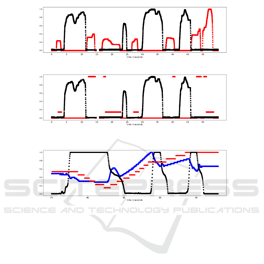
(a) Brake pedal (black) vs. accelerator pedal (red) position

(b) A false match

Figure 3: Searching for the brake and accelerator pedal position signals.

Figure 4: The clutch pedal position (black) vs. RPM (blue) vs. velocity (red) of one of our test vehicles.

form (slipping clutch) around the same time. We nar-

rowed our search to cases when the vehicle acceler-

ated from zero to at most 50 km/h. In Figure 4 we

can see these signal characteristics compared to each

other. We managed to ﬁnd the clutch pedal position

and RPM signals based on the above. As before, we

validated our ﬁndings with manual physical tryouts.

Optimization. After extracting the ground truth sig-

nals, we calculated the feature vectors and trained a

random forest classiﬁer for each extracted signal: ve-

locity, brake pedal position, accelerator pedal posi-

tion, clutch pedal position and engine RPM. For pa-

rameter optimization and testing we tested our model

on logs from the same car, but driven by another

driver on another route.

6.4 Results

Next we describe the performance of our classiﬁers

used to extract signals from CAN logs (in Section

6.4.1) and to re-identify drivers using the extracted

signals (in Section 6.4.2).

6.4.1 Signal Extraction

Our random forest classiﬁers used for signal extrac-

tion are trained on the CAN logs of a base car (here

it is an Opel Astra’18) where the locations of a target

signal is known. The classiﬁers take statistical data

vectors as inputs with the 15 statistical features (see in

Section 6.2) extracted from each sample (window). In

particular, we train a random forest classiﬁer to distin-

guish a target signal from all other signals, where the

positive training samples are composed of the win-

dows of the time series corresponding to the target

signal, whereas negative samples are taken from other

signals’ time series. Hence, we obtain a classiﬁer per

target signal. Recall that signal locations are com-

puted using the techniques described in Section 6.3.

We apply each trained classiﬁer on all the samples

(windows) of all time series in another (target) car

where we want to locate the corresponding target sig-

nals. For every classiﬁer, we obtain a classiﬁcation

for each window of each time series in the target car.

The time series which receives the largest number of

votes (i.e., has the most windows classiﬁed as posi-

Extracting Vehicle Sensor Signals from CAN Logs for Driver Re-identiﬁcation

143

tive) will be the matched signal, i.e. the signal which

is the most similar to the target signal.

Best results were obtained using the following pa-

rameter settings: the length of windows is set to 2.5

seconds, which is sufﬁciently large to capture differ-

ent driver reactions (one can accelerate from 0 to even

30 km/h or can hit the brakes and stop the vehicle).

The sampled logs are at least 30 minutes long, the

overlap parameter is set to 25%. The pruning param-

eter is set to 7, i.e. a sample was excluded when its

variation is less than 7.

Each trained random forest classiﬁer is tested

against samples from logs of all other cars except the

base car, and the logs were pre-processed as described

in Section 5.2. The matching performed by a clas-

siﬁer is validated by manually extracting the ground

truth sensor signal from the target car as described in

Section 6.3. In order to measure the accuracy of our

classiﬁer, we report the rank of the true signal; each

candidate signal is ranked according to the number of

votes (i.e., positive classiﬁcations) they receive, i.e.

the signal having the highest vote ranked ﬁrst.

Table 4 shows the results of signal extraction us-

ing only 30 minutes of data for training and also 30

minutes for matching (testing), where training was

performed on CAN logs obtained from our base car

(i.e., Opel Astra’18). Three signals (RPM, velocity

and accelerator pedal position) are all ranked in the

ﬁrst place (i.e. received the highest number of votes in

the classiﬁer),that is, our approach successfully iden-

tiﬁed all three signals in all the target cars. Note that

we did not exract the clutch and the brake pedal posi-

tion signals as during the validation we realized that

these signals do not even exist in most of our cars in

the database.

We also report the precision (TP/TP+FP) and re-

call (TP/TP+FN) of the classiﬁer (where TP=true pos-

itive, FP=false positive and FN=false negative) which

represent how many positive classiﬁcations are cor-

rect over all samples of all time-series in the CAN log

(precision), and how many samples of the true match-

ing signal are correctly recognized by the classiﬁer

(recall). We also compute and report the gap which is

the difference between the number of votes (i.e., pos-

itive classiﬁcations) of the highest ranked true signal

and that of the highest ranked false signal divided by

the total number of votes. For example if the high-

est ranked true signal received 50% of the votes and

the highest ranked false signal received 20%, then the

gap equals 0.30. Note that in most cars most sensors

appear under several IDs in the log, this causes that

more than one candidate with very high votes are all

true positives, thus the top high ranks can all be true

positives and the highest ranked false signal drops to

Table 4: Top results against RPM, velocity and acceleration.

Sensor Rank Precision Recall Gap

Citroen rpm 1 0.353 0.952 0.180

Citroen velo 1 0.874 0.792 0.094

Citroen acc 1 0.740 0.444 0.431

Opel A06 rpm 1 0.155 0.604 0.035

Opel A06 velo 1 0.158 0.969 0.024

Opel A06 acc 1 0.207 0.934 0.026

Toyota A rpm 1 0.229 0.717 0.238

Toyota A velo 1 0.230 0.214 0.337

Toyota A acc 1 0.394 0.566 0.296

Toyota C rpm 1 0.224 0.399 0.049

Toyota C velo 1 0.676 0.139 0.029

Toyota C acc 1 0.602 0.522 0.134

Renault rpm 1 0.439 0.991 0.148

Renault velo 1 0.890 0.522 0.465

Renault acc 1 0.491 0.702 0.210

Nissan X rpm 1 0.248 0.805 0.140

Nissan X velo 1 0.970 0.870 0.466

Nissan X acc 1 0.484 0.728 0.527

Nissan Q rpm 1 0.211 0.680 0.034

Nissan Q velo 1 0.462 0.522 0.110

Nissan Q acc 1 0.512 0.774 0.044

the fourth, ﬁfth or even lower places.

6.4.2 Driver Re-identiﬁcation

Next we use the extracted signals in a driver re-

identiﬁcation scenario. We use the same preprocess-

ing as in Section 5.2 and the same parameter settings

as in Section 6.3, except that we do not use all 15

features, only 11 of them are chosen based on their

importances: count above mean, count below mean,

longest strike above mean, longest strike below mean,

maximum, mean, mean abs change, median, mini-

mum, standard deviation, variance. We used four ex-

tracted signals: accelerator and brake pedal positions,

velocity and RPM. The feature vector of a driver con-

sists of 44 features altogether. All drivers used the

same car, which was Opel Astra’18, to produce CAN

logs. The samples were divided into a training and

testing set, where the training and testing data made

90% and 10% of all samples, respectively. We used

10-fold cross-validation to evaluate our approach. We

selected 5 drivers uniformly at random, and built a bi-

nary classiﬁer for each pair of drivers. Our classiﬁer

achieved 77% precision on average (each model was

evaluated 10 times). The worst result was just under

70% and the best result was 87%.

7 CONCLUSION AND FUTURE

WORK

We described a technique to extract signals from vehi-

cles’ CAN logs. Our approach relies on using unique

ICISSP 2019 - 5th International Conference on Information Systems Security and Privacy

144

statistical features of signals which remain mostly un-

changed even between different types of cars, and

hence can be used to locate the signals in the CAN

log. We demonstrated that the extracted signals can

be used to effectively identify drivers in a dataset of

33 drivers. Although our results need to be evalu-

ated on a larger and more diverse dataset, our ﬁndings

show that driver re-identiﬁcation can be performed

without the nuisance of signal extraction or agree-

ments with a manufacturer. This means that not re-

vealing the exact signal location in CAN logs is not

sufﬁcient to provide any privacy guarantee in prac-

tice. Car companies should devise more principled

(perhaps cryptographic) approaches to hide signals,

and/or to anonymize their CAN logs so that drivers

cannot be re-identiﬁed.

ACKNOWLEDGEMENTS

This work has been partially funded by the Eu-

ropean Social Fund via the project EFOP-3.6.2-

16-2017-00002, by the European Commission via

the H2020-ECSEL-2017 project SECREDAS (Grant

Agreement no. 783119) and the Higher Education

Excellence Program of the Ministry of Human Ca-

pacities in the frame of Artiﬁcial Intelligence re-

search area of Budapest University of Technology and

Economics (BME FIKP-MI/FM). Gergely Acs has

been supported by the Premium Post Doctorate Re-

search Grant of the Hungarian Academy of Sciences

(MTA). Gergely Bicz

ok has been supported by the

anos Bolyai Research Scholarship of the Hungarian

Academy of Sciences.

REFERENCES

Bagnall, A., Bostrom, A., Large, J., and Lines, J. (2016).

The great time series classiﬁcation bake off: An exper-

imental evaluation of recently proposed algorithms.

extended version. arXiv preprint arXiv:1602.01711.

Enev, M., Takakuwa, A., Koscher, K., and Kohno, T.

(2016). Automobile driver ﬁngerprinting. Proceed-

ings on Privacy Enhancing Technologies, 2016(1):34–

50.

European Union (2016a). Recital 26 of Regula-

tion (EU) 2016/679 of the European Parliament

and of the Council of 27 April 2016 on the

protection of natural persons with regard to the

processing of personal data and on the free

movement of such data, and repealing Direc-

tive 95/46/EC (General Data Protection Regulation),

OJ L119, 4.5.2016. http://eur-lex.europa.eu/legal-

content/en/TXT/?uri=CELEX%3A32016R0679.

European Union (2016b). Regulation (EU) 2016/679 of

the European Parliament and of the Council of 27

April 2016 on the protection of natural persons with

regard to the processing of personal data and on the

free movement of such data, and repealing Directive

95/46/EC (General Data Protection Regulation). Ofﬁ-

cial Journal of the European Union, L119:1–88.

Fugiglando, U., Massaro, E., Santi, P., Milardo, S., Abida,

K., Stahlmann, R., Netter, F., and Ratti, C. (2018).

Driving behavior analysis through can bus data in an

uncontrolled environment. IEEE Transactions on In-

telligent Transportation Systems, (99).

Fugiglando, U., Santi, P., Milardo, S., Abida, K., and Ratti,

C. (2017). Characterizing the driver dna through can

bus data analysis. In Proceedings of the 2nd ACM

International Workshop on Smart, Autonomous, and

Connected Vehicular Systems and Services, pages 37–

41. ACM.

Geurts, P. (2001). Pattern extraction for time series clas-

siﬁcation. In European Conference on Principles of

Data Mining and Knowledge Discovery, pages 115–

127. Springer.

Hallac, D., Sharang, A., Stahlmann, R., Lamprecht, A.,

Huber, M., Roehder, M., Leskovec, J., et al. (2016).

Driver identiﬁcation using automobile sensor data

from a single turn. In Intelligent Transportation Sys-

tems (ITSC), 2016 IEEE 19th International Confer-

ence on, pages 953–958. IEEE.

Markovitz, M. and Wool, A. (2017). Field classiﬁcation,

modeling and anomaly detection in unknown can bus

networks. Vehicular Communications, 9:43–52.

Miyajima, C., Nishiwaki, Y., Ozawa, K., Wakita, T., Itou,

K., Takeda, K., and Itakura, F. (2007). Driver mod-

eling based on driving behavior and its evaluation

in driver identiﬁcation. Proceedings of the IEEE,

95(2):427–437.

Salvador, S. and Chan, P. (2007). Toward accurate dynamic

time warping in linear time and space. Intelligent Data

Analysis, 11(5):561–580.

Sija, B. D., Goo, Y.-H., Shim, K.-S., Hasanova, H., and

Kim, M.-S. (2018). A survey of automatic protocol re-

verse engineering approaches, methods, and tools on

the inputs and outputs view. Security and Communi-

cation Networks, 2018.

Szalay, Z., K

anya, Z., Lengyel, L., Ekler, P., Ujj, T.,

Balogh, T., and Charaf, H. (2015). Ict in road ve-

hicles—reliable vehicle sensor information from obd

versus can. In Models and Technologies for Intelligent

Transportation Systems (MT-ITS), 2015 International

Conference on, pages 469–476. IEEE.

Voss, W. (2008). A comprehensible guide to controller area

network. Copperhill Media.

Extracting Vehicle Sensor Signals from CAN Logs for Driver Re-identiﬁcation

145