Circular Fringe Projection Method for

3D Proﬁling of High Dynamic Range Objects

Jagadeesh Kumar Mandapalli

, Sai Siva Gorthi

, Ramakrishna Sai Gorthi

and Subrahmanyam Gorthi

Department of Electrical Engineering, Indian Institute of Technology, Tirupati, Andhra Pradesh, 517506, India

Department of Instrumentation and Applied Physics, Indian Institute of Science, Bangalore, 560012, India

Keywords:

3D Shape Measurement, Fourier Transform, Fringe Projection, High Dynamic Range.

Abstract:

Fringe projection proﬁlometry is a widely used active optical method for 3D proﬁling of real-world objects.

Linear fringes with sinusoidal intensity variations along the lateral direction are the most commonly used

structured pattern in fringe projection proﬁlometry. The structured pattern, when projected onto the object of

interest gets deformed in terms of phase modulation by the object height proﬁle. The deformed fringes are

demodulated using methods like Fourier transform proﬁlometry for obtaining the wrapped phase information,

and the unwrapped phase provides the 3D proﬁle of the object. One of the key challenges with the conventional

linear fringe Fourier transform proﬁlometry (LFFTP) is that the dynamic range of the object height that can

be measured with them is very limited.

In this paper we propose a novel circular fringe Fourier transform proﬁlometry (CFFTP) method that uses

circular fringes with sinusoidal intensity variations along the radial direction as the structured pattern. A new

Fourier transform-based algorithm for circular fringes is also proposed for obtaining the height information

from the deformed fringes. We demonstrate that, compared to the conventional LFFTP, the proposed CFFTP

based structure assessment enables 3D proﬁling even at low carrier frequencies, and at relatively much higher

dynamic ranges. The reasons for increased dynamic range with circular fringes stem from the non-uniform

sampling and narrow band spectrum properties of CFFTP. Simulation results demonstrating the superiority of

CFFTP over LFFTP are also presented.

1 INTRODUCTION

3D shape reconstruction techniques are widely used

in various ﬁelds like industrial automation, compu-

ter vision, and medical imaging. Among the availa-

ble methods, fringe projection technique is a com-

monly used active optical method (Gorthi and Ra-

stogi, 2010) for 3D proﬁling because of its righte-

ous properties like non-contact based non-destructive

operation and its ability to give high resolution. Furt-

hermore, with the fringe projection technique, the 3D

shape of an object can be reconstructed from a single

image, and thus it can be used for real time 3D shape

measurements.

Fig. 1 shows a typical experimental set-up used in

fringe projection technique. A structured pattern, usu-

ally linear fringes with sinusoidal intensity variation

along the lateral direction, is projected onto the object

of interest. The projected pattern gets phase modula-

ted in accordance with the object height proﬁle (or

depth proﬁle), and it is recorded with a camera. The

recorded pattern is phase-demodulated and the result

is unwrapped for obtaining the actual height of the

object at each pixel location.

Several methods have been developed in the lite-

rature for phase demodulation, e.g., Fourier transform

proﬁlometry (Takeda and Mutoh, 1983; Lin and Su,

1995; Su and Chen, 2001), windowed Fourier trans-

form proﬁlometry (Kemao, 2004; Kemao, 2007),

spatial phase detection method (Toyooka and Iwaasa,

1986; Sajan et al., 1998), and wavelet transform met-

hod (Dursun et al., 2004; Zhong and Weng, 2004;

Gdeisat et al., 2006). Since phase demodulation met-

hods result in wrapped phase whose values are map-

ped to the range [−π, π), these are generally followed

by a phase unwrapping procedure. Phase unwrap-

ping is performed using methods like ZπM (Dias and

Leit

ao, 2002), Goldstein’s phase unwrapping (Gold-

stein et al., 1988), branch cut (Gutmann and Weber,

2000), ﬂood ﬁll (Asundi and Wensen, 1998), region

Mandapalli, J., Gorthi, S., Gorthi, R. and Gorthi, S.

Circular Fringe Projection Method for 3D Proﬁling of High Dynamic Range Objects.

DOI: 10.5220/0007389608490856

In Proceedings of the 14th International Joint Conference on Computer Vision, Imaging and Computer Graphics Theory and Applications (VISIGRAPP 2019), pages 849-856

ISBN: 978-989-758-354-4

849

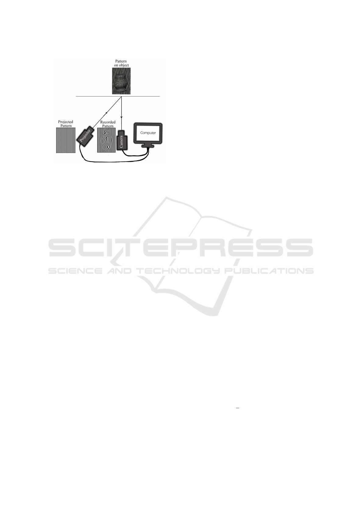
Figure 1: Schematic diagram illustrating the principle of

fringe projection proﬁlometry. Structured pattern generated

in the computer is projected onto the object (lying on refe-

rence plane) through the projector and the phase modulated

pattern is captured through the camera for further analysis.

growing phase unwrapping (Baldi, 2003), regularized

phase tracking (Servin et al., 1999), and multilevel

quality guided phase unwrapping algorithm (Zhang

et al., 2007). It can be noted that the aforementi-

oned phase-demodulation algorithms are applicable

only for linear fringes.

Various types of structured patterns have been pro-

posed in the literature for fringe projection proﬁlome-

try. Typically, the intensity proﬁles of these structu-

red patterns are repetitive along the lateral direction.

Linear fringes having sinusoidal intensity proﬁle al-

ong the lateral direction are the most commonly used

fringe pattern (Gorthi and Rastogi, 2010). Other

types of patterns include hexagonal grating (Iwata

et al., 2008), linear fringes with triangular intensity

proﬁle (Jia et al., 2008) and sawtooth intensity pro-

ﬁle (Chen et al., 2005) along the lateral direction.

In this paper, we propose a novel circular fringe-

based proﬁlometry that employs circular fringes with

sinusoidal intensity variations along the radial di-

rection as the structured pattern. We also propose a

new approach for quantifying the underlying phase

of the radially varying circular fringes. Unlike the

existing linear fringe Fourier transform proﬁlome-

try (LFFTP), the use of circular fringes in the pro-

posed circular fringe Fourier transform proﬁlometry

(CFFTP) have several advantages like relatively more

accurate 3D proﬁling of the objects at lower carrier

frequencies and even at high dynamic range of the ob-

ject height proﬁle. All these aspects are presented in

detail in the rest of this paper. We note that (Zhao

et al., 2016) have used circular fringes with sinusoi-

dal intensity variations along radial direction. But it is

used for a different purpose of coming up with a new

hardware conﬁguration of camera and projector set-

up, for obtaining a simpliﬁed calibration of 3D height

and thus it does not include any algorithms or analysis

for dealing with circular fringe pattern.

The rest of the paper is organized as follows.

Section 2 presents the details of the existing and pro-

posed methods. Section 3 presents a detailed evalua-

tion of the proposed method. Finally, conclusions are

presented in section 4.

2 METHODOLOGY

This section ﬁrst presents the details of the exis-

ting Linear Fringe Fourier Transform Proﬁlometry

(LFFTP). It is then followed by the details of the pro-

posed Circular Fringe Fourier Transform Proﬁlome-

try (CFFTP).

2.1 Existing Linear Fringe Fourier

Transform Proﬁlometry

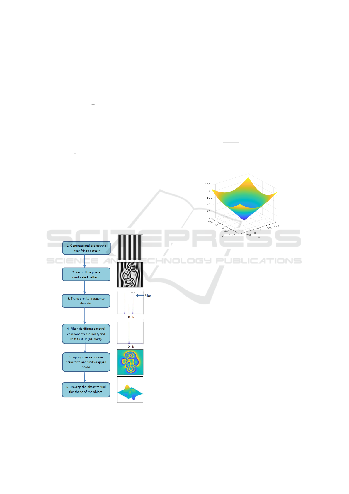
The sequence of steps followed for 3D proﬁling with

LFFTP is depicted with the aid of Fig. 2 along with

illustrative ﬁgures at each stage. The intensity proﬁle

of the projected pattern in LFFTP (step 1 of Fig. 2) is

(x, y) = a(x, y) + b(x, y) cos(2π f

x + Φ

)

where f

is the carrier or fringe frequency, (x, y) are

the spatial coordinates, a represents intensity variati-

ons in the background, b represents the non-uniform

reﬂectivity of the diffusely reﬂecting object and Φ

the initial phase (assumed to be zero).

The intensity proﬁle of the recorded phase modu-

lated pattern (step 2 of Fig. 2) is

(x, y) = a(x, y) + b(x, y) cos(2π f

x + Φ

(x, y)).

(1)

(x, y) in Eq. 1 is the phase term introduced by

the object height proﬁle. In fringe projection techni-

que, generally the underlying phase term in the phase

modulated pattern contains the information about the

shape of the object. Any of the fringe analysis techni-

ques mentioned in the preceding section can be used

on the modulated pattern for quantifying the under-

lying phase term. For ease of analysis, rewriting Eq. 1

in terms of complex exponentials using Euler formula

gives

(x, y) = a(x, y) +

[c(x, y)e

j2π f

+ c

∗

(x, y)e

− j2π f

]

(2)

where c(x , y) = b(x , y) e

jΦ

(x,y)

for real b(x,y), and

∗

indicates conjugate of c. The desired parameter

(x, y) can be found by retrieving either c(x, y) or

VISAPP 2019 - 14th International Conference on Computer Vision Theory and Applications

850

∗

(x, y) from Eq. 2. LFFTP achieves the same by

applying Fourier transform analysis. In LFFTP, the

phase modulated pattern (I

(x, y)) is ﬁrst transformed

to Fourier domain (step 3 of Fig. 2). Fourier domain

representation of Eq. 2 is

F {I

} = A( f

, f

[C( f

− f

, f

)+C

∗

( f

+ f

, f

)]

(3)

where F represents Fourier transform. As

a(x, y) represents background intensity variations, the

spectrum of A( f

, f

) will be in the low frequency

region. The spectral components around carrier fre-

quency ( f

) are extracted using a bandpass ﬁlter, and

is given by

C( f

− f

, f

). The ﬁltered spectrum

is then DC shifted (step 4 of Fig. 2), i.e., the re-

sultant spectrum is shifted such that the dominant

spectral component which was previously occurring

at f

, occurs now at zero Hertz. The result of DC shift

C( f

, f

The phase function found after the application of

inverse Fourier transform on the DC shifted signal is

wrapped (step 5 of Fig. 2) in the interval [−π, π). On

unwrapping (step 6 of Fig. 2), the result gives the 3D

proﬁle of the object of interest.

Figure 2: Block diagram illustrating the existing linear

fringe Fourier transform proﬁlometry (LFFTP) algorithm.

2.2 Proposed Circular Fringe Fourier

Transform Proﬁlometry

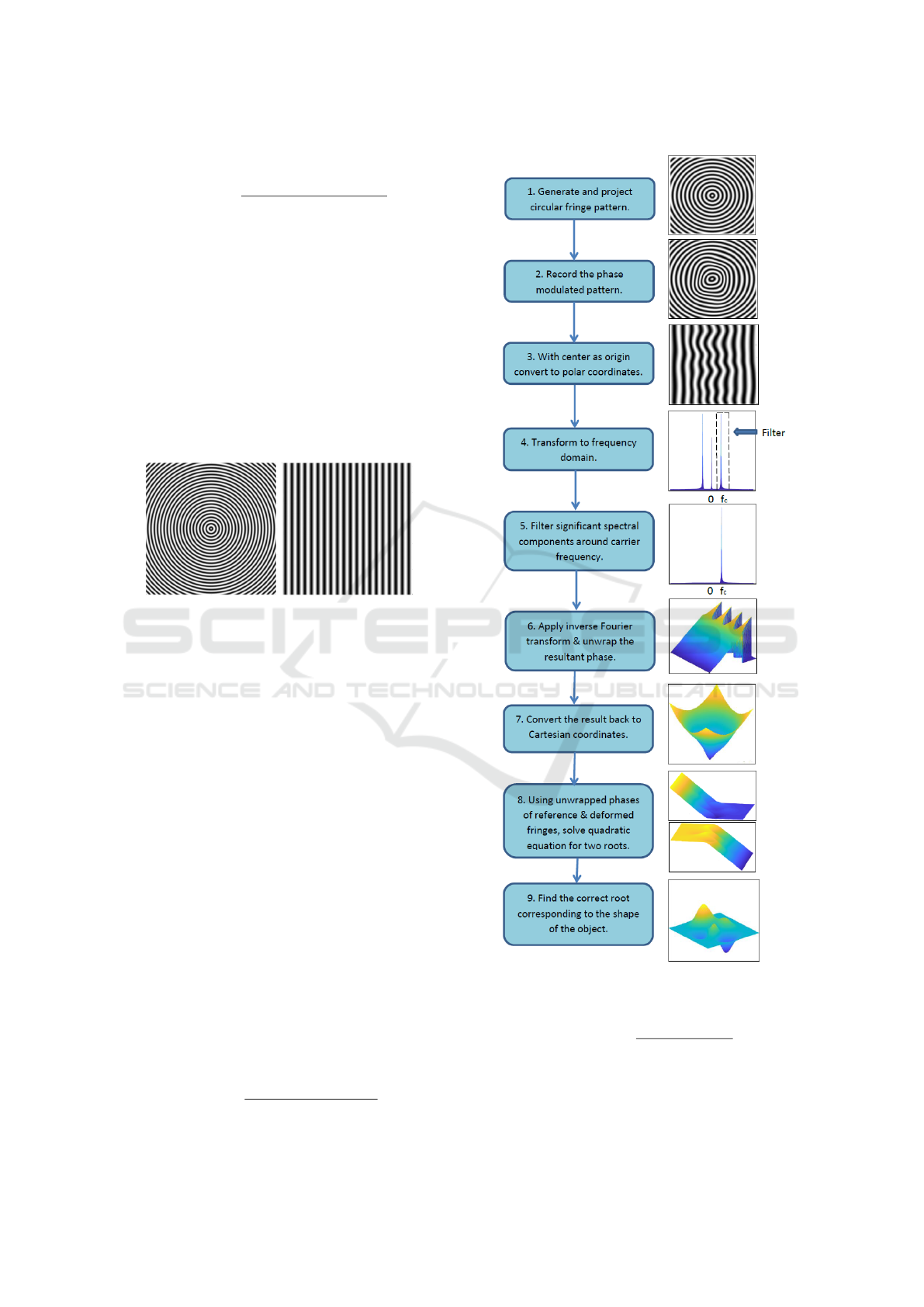
The sequence of steps required for 3D proﬁling with

CFFTP is depicted with the aid of Fig. 5 along with

illustrative ﬁgures at each stage. In CFFTP, the in-

tensity proﬁle of the circular fringe pattern projected

onto the object (step 1 of Fig. 5) is

(x, y) = a(x, y) + b(x, y) cos(2π f

+ y

). (4)

Let φ

(x, y) represent the argument of the cos

function in the above projection equation, i.e., let

(x, y) = 2π f

+ y

. Notice that φ

(x, y) has the

shape of a cone for varying values of x and y as shown

in Fig. 3. The minimum value of φ

(x, y) is zero, and

it occurs at the origin.

Figure 3: Phase function (φ

(x, y)) of the projected pattern.

It has the shape of a cone with a minimum values of zero at

origin.

When the aforementioned circular fringe pattern

is projected onto the object of interest, based on the

height proﬁle of the object at that point, the pattern

accordingly gets shifted in the x direction. Hence, the

intensity proﬁle of the recorded phase modulated pat-

tern in CFFTP (step 2 of Fig. 5) is given by:

(x, y) = a(x, y)+b(x, y) cos(2π f

(x + δ

(x))

+ y

(5)

Let φ

(x, y) represent the phase function associa-

ted with the above recorded pattern, and is given by

(x, y) = 2π f

(x + δ

(x))

+ y

. Note that φ

(x, y)

differs with φ

(x, y) in terms of the modulating term

(x). It can be noted that while the vortex of the pro-

jected pattern is at the origin, it is shifted by a value of

(0) along the x-axis for the recorded pattern. δ

(x)

is introduced due to the object height proﬁle, and thus

it contains the information about the shape of the ob-

ject. δ

(x) can be recovered from φ

(x, y) if f

, x and

y are known. Fringe frequency ( f

) is engineering

choice and is known. The parameters x and y present

in φ

(x, y) can be used to ﬁnd δ

(x) from φ

(x, y). Sol-

ving the phase functions φ

(x, y) and φ

(x, y) for δ

(x)

Circular Fringe Projection Method for 3D Proﬁling of High Dynamic Range Objects

851

results in the following quadratic equation in δ

(x):

(x) + 2x δ

(x) +

(φ

(x, y))

− (φ

(x, y))

(2π f

)

= 0 (6)

The above quadratic equation results in two roots, and

one of them corresponds to the height proﬁle of the

object. The procedure for ﬁnding out the actual root

that corresponds to the object height is presented in

the later part of this section.

As stated earlier, all the fringe analysis algorithms

mentioned in section 1 are designed for linear fringes,

and they cannot be directly applied for circular frin-

ges. However, as illustrated in Fig. 4, circular frin-

ges in the rectangular coordinates become linear frin-

ges in the polar coordinates. Hence, any of the linear

fringe analysis methods can be applied after transfor-

ming circular fringes into polar coordinates.

(a) Circular fringes (b) Polar equivalent of

circular fringes

Figure 4: Circular fringes in Cartesian coordinates and their

polar equivalents. Horizontal axis in polar representation is

radius r and vertical axis is angle θ.

The proposed algorithm for retrieving the true

phase of the recorded fringe pattern

Proposed Algorithm for Phase Retrieval

1. As discussed above, in order to be able to ap-

ply any of the existing linear fringe analysis

algorithms, the circular fringe has to be ﬁrst

transformed into polar coordinates by considering

the centre of the circular fringes as the origin.

To this end, the centre of the recorded circular

fringe is computed, and the coordinate transfor-

mation is applied. The centre of the recorded

circular fringe in our experiments is computed

using ‘imﬁndcircles’ function in MATLAB. Let

, 0) represent the centre of the recorded circular

fringe. Then the equation representing the recor-

ded fringe transformed into the polar coordinates

is given by:

, θ) = a(r

, θ) + b(r

, θ) cos(2π f

), (7)

where

(x − x

+ δ

(x))

+ y

Figure 5: Block diagram illustrating the proposed circular

fringe Fourier transform proﬁlometry (CFFTP) algorithm.

θ = tan

−1



(x − x

+ δ

(x))



The result of this polar coordinates transformation

is illustrated in step 3 of Fig. 5.

2. Fourier transform proﬁlometry is applied on the

VISAPP 2019 - 14th International Conference on Computer Vision Theory and Applications

852

fringe pattern represented by Eq. 7. The resulting

frequency domain representation is given by:

F {I

} = A( f

, f

) +

B( f

− f

, f

B( f

+ f

, f

). (8)

Step 4 of Fig. 5 illustrates the resulting magnitude

spectrum.

3. The spectral components around carrier frequency

are extracted using a bandpass ﬁlter. The result of

bandpass ﬁltering is given by

B( f

− f

, f

), and

it is illustrated in step 5 of Fig. 5.

4. Inverse Fourier transform is applied on the output

of the bandpass ﬁlter, and the result is given by:

b(r

, θ) e

j2π f

. As discussed in section 1, the

resultant phase of the above expression is wrap-

ped into the range [−π, π). It is then unwrapped

using any of the phase unwrapping methods, and

is illustrated in step 6 of Fig. 5.

5. The unwrapped phase is transformed back into

Cartesian coordinates to get φ

(x, y), and is illus-

trated in step 7 of Fig. 5.

The above mentioned algorithm can extract

(x, y), φ

(x, y), and the remaining task now is to

compute δ

(x) based on Eq. 6.

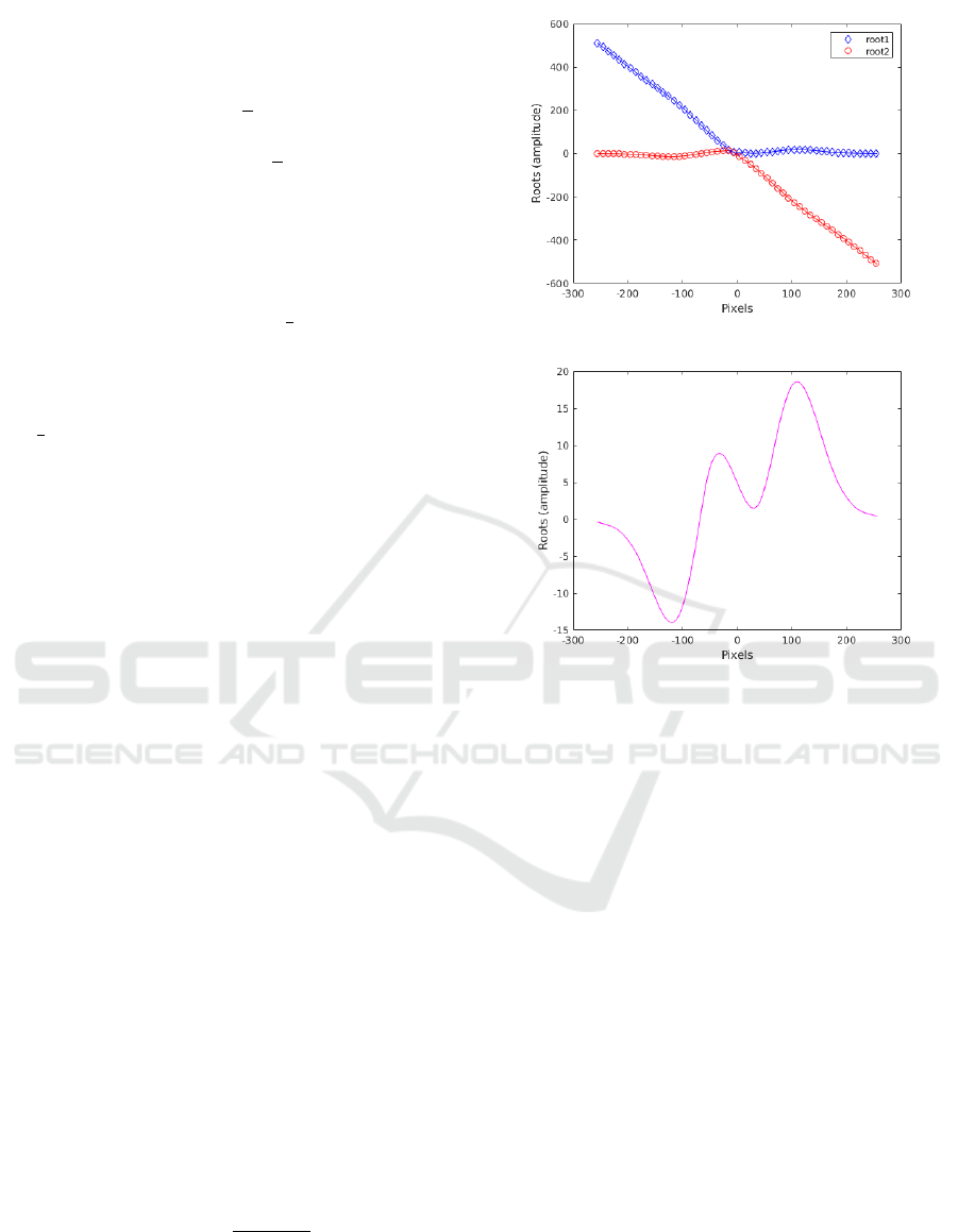
Solving the quadratic Eq. 6 for each row (y), by

substituting φ

and φ

, gives two roots for δ

(x) as

shown in step 8 of Fig. 5. Two such roots found from

Eq. 6 for one of the rows are shown in Fig. 6(a). The

actual root that corresponds to the height proﬁle of the

object is obtained by imposing the following two con-

straints. Firstly, it is considered that the height proﬁle

is continuous over neighbourhood spatial locations.

Secondly, the difference in the position of vortices of

(x, y) and φ

(x, y) is relatively nearer to the average

value of the object height proﬁle. Fig. 6(b) shows the

actual root extracted from the two roots displayed in

Fig. 6(a) after imposing the above constraints. Ap-

plying the same procedure for all the rows gives the

actual root corresponding to the shape of the object as

shown in step 9 of Fig. 5.

Finally, after the computation of δ

(x), the actual

height proﬁle of the object is obtained using the fol-

lowing calibration equation (Zhang et al., 2002)

H(x, y) =

k δ

(x)

d − δ

(x)

(9)

where k is the distance between the camera and re-

ference plane, d is the baseline distance between the

camera and projector.

(a) Roots obtained by solving the quadratic Eq. 6.

(b) Actual root extracted form the two roots.

Figure 6: Illustration of the two roots obtained by solving

Eq. 6 for one of the rows, and the extracted actual root that

corresponds to the height proﬁle of the object.

3 RESULTS

In this section, we present a comparison of the results

from the proposed circular fringe projection based

method (CFFTP) with the results from the existing li-

near fringe projection based method (LFFTP). More

speciﬁcally, the accuracies of the CFFTP and LFFTP

methods are evaluated for varying dynamic range of

the objects, and also for varying fringe frequencies.

The evaluations are performed on simulated data

with varying shapes and dynamic ranges. Various

shapes are generated through Gaussian Mixture Mo-

dels (GMM) by randomly choosing the locations of

the peaks and valleys with the help of a random num-

ber generator. Fig. 7 shows samples of such randomly

generated object height proﬁles. While performing

evaluations for varying dynamic range, those rand-

omly generated shapes are scaled accordingly.

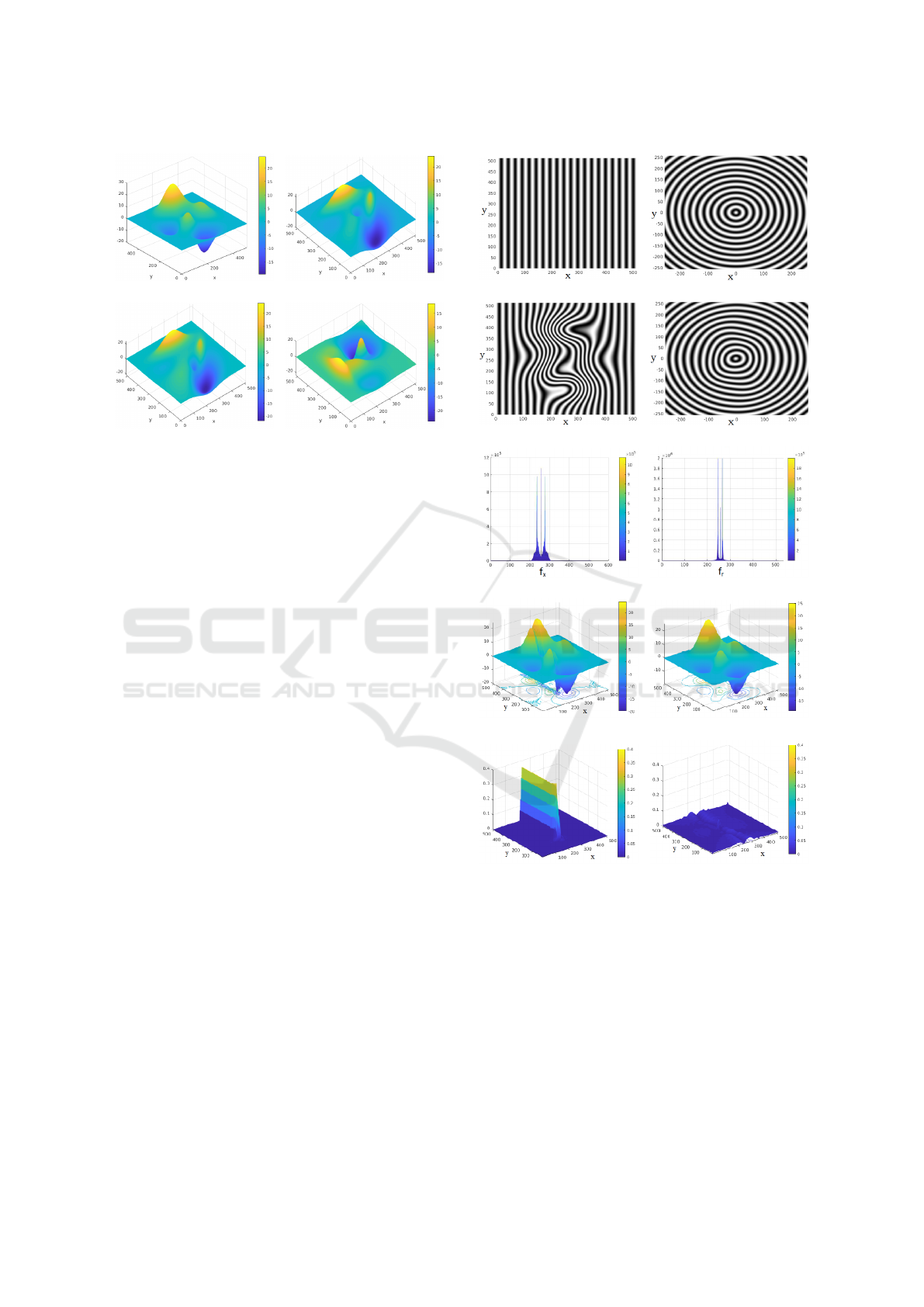
Fig. 8 shows the results obtained from LFFTP and

CFFTP when reconstructing the height proﬁle of the

simulated object shown in Fig. 7(a). The fringe fre-

Circular Fringe Projection Method for 3D Proﬁling of High Dynamic Range Objects

853

(a) (b)

Figure 7: Sample simulated objects with arbitrary height

proﬁles.

quency and the dynamic range values used for this

particular evaluation are 20 Hz and ±24 pixels re-

spectively. The left and the right columns of this ﬁ-

gure present the results from the LFFTP and CFFTP

respectively. First row in Fig. 8 shows the projected

patterns. Second row of the same ﬁgure shows the

modulated patterns in LFFTP and CFFTP. Fig. 8(e) is

the magnitude spectrum of the deformed linear fringe

pattern, and Fig. 8(f) is the magnitude spectrum of the

deformed circular fringe pattern after transforming

it into polar coordinates. It can be observed from

Fig. 8(e) and Fig. 8(f) that for a given height proﬁle

of the object, the spectral variations in the magnitude

spectrum of LFFTP are relatively more than that of in

CFFTP. Fig. 8(g) and Fig. 8(h) show 3D proﬁling re-

sults obtained from LFFTP and CFFTP respectively.

In order to quantify the accuracies of the results

from LFFTP and CFFTP, the difference between the

ground truth and the reconstructed output from these

methods are computed at each pixel. These values are

normalized by dividing with the dynamic range (i.e.,

the difference between the maximum and minimum

values of the ground truth). Fig. 8(i) and Fig. 8(j)

show the resulting error plots for LFFTP and CFFTP

respectively. Maximum normalized error values are

found to be 0.37 for LFFTP, and 0.064 for CFFTP.

Thus, the proposed CFFTP resulted in more accurate

3D reconstruction compared to the existing LFFTP.

We have also studied the effects of varying the dy-

namic range on the magnitude spectrums of LFFTP

and CFFTP. Fig. 9 presents the magnitude spectrums

of LFFTP and CFFTP for varying dynamic range. It

can be observed from these results that for the propo-

sed CFFTP, aliasing in frequency domain is starting

to occur at relatively high dynamic range values than

(a) (b)

(e) (f)

(g) (h)

(i) (j)

Figure 8: Simulation results from the existing LFFTP and

the proposed CFFTP are presented in the ﬁrst and second

columns respectively. Projected fringes, deformed fringes,

magnitude spectrum, reconstructed object height proﬁles,

and normalized error values are presented in rows 1, 2, 3, 4,

and 5 respectively.

that LFFTP. Because of such narrowband properties

of CFFTP, it is able to more accurately reconstruct the

3D proﬁles of the objects having high dynamic range

than LFFTP.

Fig. 10 shows the effect of varying the dynamic

range on the 3D reconstruction results of LFFTP and

CFFTP. For this purpose, all the height proﬁles shown

VISAPP 2019 - 14th International Conference on Computer Vision Theory and Applications

854

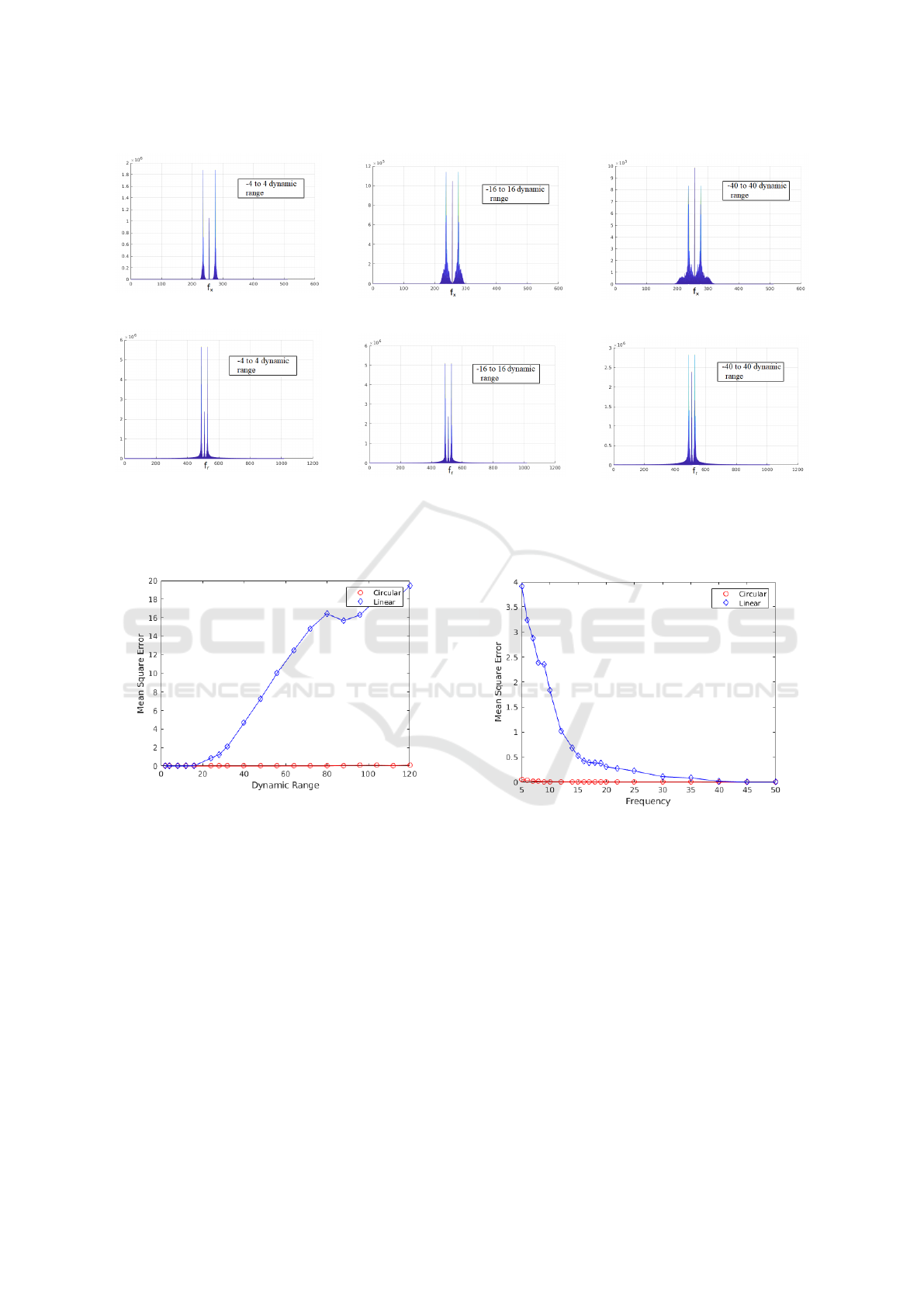
(a) LFFTP with a dynamic range of

±4.

(b) CFFTP with a dynamic range of

±4.

±16.

(d) CFFTP with a dynamic range of

±16.

(e) LFFTP with a dynamic range of

±40.

(f) CFFTP with a dynamic range of

±40.

Figure 9: Illustration of spectral changes in the magnitude spectrums of the LFFTP and the proposed CFFTP with varying

dynamic range.

Figure 10: Plot of normalized MSE showing the compara-

tive performance of LFFTP and CFFTP for increasing dyna-

mic range of the object height. CFFTP has low normalized

MSE at high dynamic ranges of object height for a fringe

frequency of 20 Hz.

in Fig. 7 are considered, and Mean Square Error

(MSE) values presented in Fig. 10 are the averaged

values computed across all the datasets. Some of the

intermediate MSE values corresponding to this evalu-

ation are presented in Table 1. Notice that if the nor-

malized MSE value is 0.85, it means that the MSE is

85% of the dynamic range of the object height. Thus,

CFFTP is found to result in signiﬁcantly lower error

values than the existing LFFTP, particularly at high

dynamic range values. Finally, Fig. 11 shows norma-

lized MSE values for varying fringe frequencies, for

a dynamic range of ±24. Similar to the preceding ex-

periment, MSE values are averaged across all the da-

Figure 11: Plot of normalized MSE showing the compa-

rative performance of LFFTP and CFFTP for increasing

fringe frequency. CFFTP has low normalized MSE at low

fringe frequency for a dynamic range of ±24.

tasets. It can be observed that while both LFFTP and

CFFTP perform equally well at high frequencies, the

proposed CFFTP signiﬁcantly outperforms LFFTP at

low frequencies.

4 CONCLUSIONS

In this paper, we have presented a new circular fringe

Fourier transform proﬁlometry (CFFTP) method for

3D proﬁling of objects. Unlike the conventional linear

fringes, the proposed method uses circular fringes

Circular Fringe Projection Method for 3D Proﬁling of High Dynamic Range Objects

855

Table 1: Normalized MSE values in case of LFFTP and

CFFTP for increasing dynamic range of object height.

Dynamic range of Normalized MSE

the object height LFFTP CFFTP

± 4 0.00 0.00

± 8 0.00 0.00

± 16 0.02 0.00

± 24 0.85 0.00

± 40 4.66 0.00

± 56 10.01 0.00

± 80 16.43 0.01

± 120 19.44 0.10

± 160 18.06 5.83

with sinusoidal intensity variations along the radial

direction. A new algorithm is also proposed for retrie-

ving the phase information from the circular fringes.

The proposed CFFTP has been evaluated for varying

dynamic ranges and fringe frequencies. It is found

that the proposed algorithm signiﬁcantly outperforms

the existing LFFTP, particularly at high dynamic ran-

ges and low fringe frequencies. In the future work,

we plan to evaluate the proposed CFFTP method for

the 3D proﬁling of the real-world objects.

REFERENCES

Asundi, A. and Wensen, Z. (1998). Fast phase-unwrapping

algorithm based on a gray-scale mask and ﬂood ﬁll.

Applied optics, 37(23):5416–5420.

Baldi, A. (2003). Phase unwrapping by region growing.

Applied optics, 42(14):2498–2505.

Chen, L., Quan, C., Tay, C. J., and Fu, Y. (2005). Shape me-

asurement using one frame projected sawtooth fringe

pattern. Optics communications, 246(4-6):275–284.

Dias, J. M. and Leit

ao, J. M. (2002). The ZπM algorithm:

a method for interferometric image reconstruction in

SAR/SAS. IEEE Transactions on Image processing,

11(4):408–422.

Dursun, A.,

Ozder, S., and Ecevit, F. N. (2004). Conti-

nuous wavelet transform analysis of projected fringe

patterns. Measurement Science and Technology,

15(9):1768.

Gdeisat, M. A., Burton, D. R., and Lalor, M. J. (2006). Spa-

tial carrier fringe pattern demodulation by use of a

two-dimensional continuous wavelet transform. Ap-

plied optics, 45(34):8722–8732.

Goldstein, R. M., Zebker, H. A., and Werner, C. L. (1988).

Satellite radar interferometry: Two-dimensional phase

unwrapping. Radio science, 23(4):713–720.

Gorthi, S. S. and Rastogi, P. (2010). Fringe projection

techniques: whither we are? Optics and lasers in en-

gineering, 48(IMAC-REVIEW-2009-001):133–140.

Gutmann, B. and Weber, H. (2000). Phase unwrapping with

the branch-cut method: role of phase-ﬁeld direction.

Applied optics, 39(26):4802–4816.

Iwata, K., Kusunoki, F., Moriwaki, K., Fukuda, H., and

Tomii, T. (2008). Three-dimensional proﬁling using

the fourier transform method with a hexagonal grating

projection. Applied optics, 47(12):2103–2108.

Jia, P., Kofman, J., and English, C. (2008). Error com-

pensation in two-step triangular-pattern phase-shifting

proﬁlometry. Optics and Lasers in Engineering,

46(4):311–320.

Kemao, Q. (2004). Windowed fourier transform for fringe

pattern analysis. Applied Optics, 43(13):2695–2702.

Kemao, Q. (2007). Two-dimensional windowed fourier

transform for fringe pattern analysis: principles, ap-

plications and implementations. Optics and Lasers in

Engineering, 45(2):304–317.

Lin, J.-F. and Su, X. (1995). Two-dimensional fourier trans-

form proﬁlometry for the automatic measurement of

three-dimensional object shapes. Optical Engineer-

ing, 34(11):3297–3303.

Sajan, M., Tay, C., Shang, H., and Asundi, A. (1998). Im-

proved spatial phase detection for proﬁlometry using a

tdi imager. Optics communications, 150(1-6):66–70.

Servin, M., Cuevas, F. J., Malacara, D., Marroquin, J. L.,

and Rodriguez-Vera, R. (1999). Phase unwrapping

through demodulation by use of the regularized phase-

tracking technique. Applied Optics, 38(10):1934–

1941.

Su, X. and Chen, W. (2001). Fourier transform proﬁlo-

metry:: a review. Optics and lasers in Engineering,

35(5):263–284.

Takeda, M. and Mutoh, K. (1983). Fourier transform proﬁ-

lometry for the automatic measurement of 3-d object

shapes. Applied optics, 22(24):3977–3982.

Toyooka, S. and Iwaasa, Y. (1986). Automatic proﬁlome-

try of 3-d diffuse objects by spatial phase detection.

Applied Optics, 25(10):1630–1633.

Zhang, C., Huang, P. S., and Chiang, F.-P. (2002). Mi-

croscopic phase-shifting proﬁlometry based on digi-

tal micromirror device technology. Applied optics,

41(28):5896–5904.

Zhang, S., Li, X., and Yau, S.-T. (2007). Multilevel

quality-guided phase unwrapping algorithm for real-

time three-dimensional shape reconstruction. Applied

optics, 46(1):50–57.

Zhao, H., Zhang, C., Zhou, C., Jiang, K., and Fang, M.

(2016). Circular fringe projection proﬁlometry. Optics

letters, 41(21):4951–4954.

Zhong, J. and Weng, J. (2004). Spatial carrier-fringe pat-

tern analysis by means of wavelet transform: wavelet

transform proﬁlometry. Applied optics, 43(26):4993–

4998.

VISAPP 2019 - 14th International Conference on Computer Vision Theory and Applications

856