A Heuristic Method for the Multi-skill Project Scheduling Problem with

Partial Preemption

Oliver Polo-Mej

ıa

1,2

, Christian Artigues

and Pierre Lopez

CEA, DEN, DEC, SETC, St. Paul lez Durance, France

LAAS-CNRS, Universit

e de Toulouse, CNRS, Toulouse, France

Keywords:

Project Scheduling, Multi-skill, Partial Preemption, Nuclear Research Facility.

Abstract:

In this article we consider a new scheduling problem known as the Multi-Skill Project Scheduling Problem

with Partial Preemption. The main characteristic of this problem is the way we handle the resources release

during the preemption periods: only a subset of resources are released. Since this problem is NP-hard, we

propose a greedy algorithm based on priority rules, modeling the subproblem of technicians allocation as a

Minimum-Cost Maximum-Flow problem. In order to improve the performance of the greedy algorithm, we

propose a randomized tree-based local search algorithm. Computational tests are carried out and analyzed.

1 INTRODUCTION

Scheduling activities within a research nuclear facil-

ity is a very complex task. This is due to the diver-

sity of activities to schedule, and to the big amount

of constraints we must take into account in order to

complain with the operational and legal regulations.

Because of this complexity, this research project is

carried out in order to optimize the weekly schedul-

ing within one of the research facilities of the French

Alternative Energies and Atomic Energy Commission

(CEA in short for French). After a deep analysis of

the characteristics of the studied facility, we conclude

that the problem at hand can be regarded as an exten-

sion of the Multi-Skill Project Scheduling Problem.

The Multi-Skill Project Scheduling Problem

(MSPSP) acquires great importance for scheduling

activities in very speciﬁc ﬁelds, such as pharmaceu-

tical, chemical and nuclear, where the regulation re-

quires the presence of a group of technicians having

a set of well-deﬁned competences for the execution

of an activity. This problem shows to be more chal-

lenging than traditional scheduling problems (such as

the Resource-Constrained Project Scheduling Prob-

lem (Artigues, 2008)) due to the extra decision we

need to make: we need to decide not only which

resources will be assigned to each activity, but also

the skills with which they will contribute(Correia and

Saldanha-da Gama, 2015).

This problem consists in determining a feasible

schedule, respecting the resource constraints and the

precedence constraints between activities: a resource

cannot execute a skill it does not master, cannot be as-

signed to more than one competence requirement at a

given time, and must be assigned to the corresponding

activity during its whole processing time (Bellenguez-

Morineau, 2008).

One of the most important hypothesis of the

MSPSP is that activities are supposed to be non-

preemptive; what means that, once started, an activity

must run continuously until its completeness. How-

ever, in some practical applications as in the case of

scheduling research or engineering activities, it may

be interesting to allow the preemption of activities,

due for example to the impossibility of working con-

tinuously and other technical constraints. In order to

better represent the real situation of the nuclear lab-

oratory, we proposed in (Polo-Mej

ıa et al., 2018) a

more general variant of the MSPSP: the Multi-Skill

Project Scheduling Problem with Partial Preemption.

The remainder of the paper is as follows. In Sec-

tion 2, we describe the studied problem. Then, a

priority-based heuristic method is proposed in Sec-

tion 3. The computational experiments performed are

presented in Section 4. Finally, in Section 5, the main

conclusions are presented as well as some directions

for future research.

Polo-Mejía, O., Artigues, C. and Lopez, P.

A Heuristic Method for the Multi-skill Project Scheduling Problem with Partial Preemption.

DOI: 10.5220/0007390001110120

In Proceedings of the 8th International Conference on Operations Research and Enterprise Systems (ICORES 2019), pages 111-120

ISBN: 978-989-758-352-0

111

2 PROBLEM DESCRIPTION

The main drawback of preemptive versions of vari-

ous scheduling models is that activities can be pre-

empted and continued later without any additional

cost (Ballest

ın et al., 2008). The possibility of re-

suming a preempted activity without any cost does

not appear realistic enough for industrial applications

(Ballest

ın et al., 2009; Vanhoucke, 2008), due mainly

to the cost/time of setup for resuming or simply to the

reduction in the production rate.

In real life, setup time of an activity is almost

always related to only a subset of resources, while

the others can be easily preempted with insigniﬁcant

setup time. When working with preemptive schedul-

ing problem, we commonly assume that all resources

are released during the preemption periods. What we

propose in this new variant is to handle the preemp-

tion in a different way: during the preemption periods

we will release only those resources with a low setup

time while seizing those with an important setup time.

This is what we call partial preemption (Polo-Mej

ıa

et al., 2018).

In our practical case, partial preemption also an-

swers to a technical requirement for the good opera-

tion of the facility. In fact, some critical activities re-

quire the presence of equipment to ensure the conﬁne-

ment of the irradiated material or even to ensure an

inert atmosphere within this conﬁnement. For safety

reasons, the equipment ensuring these functions must

be allocated to the activity from the beginning to the

end without interruption. The remainder resources,

however, can be preempted without problem. If we

use a traditional preemptive/non-preemptive schedul-

ing approach, these activities must be deﬁned as “non-

preemptive” in order to respect the safety require-

ments. Using the concept of partial preemption, we

can better exploit the characteristics of these activities

while complying with all the operational constraints.

In the MSPSP with partial preemption (MSPSP-

PP), additionally to the characteristics of the classical

MSPSP, we must indicate for each activity the subset

of resources that can be released during the preemp-

tion periods. Preemption is now handled in three lev-

els according to the activities characteristics: 1) Non-

preemption, for activities where none of the resources

can be preempted; 2) Partial preemption, for activities

where a subset of resources can be preempted; and 3)

Full preemption, for activities where all resources can

be preempted.

Additional changes must be included in order to

better represent the research facility behavior:

• Resources in the MSPSP, as deﬁned in (N

eron,

2002), are supposed to be disjunctive, which

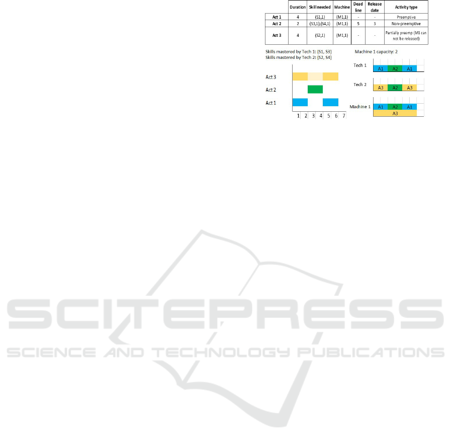
Figure 1: Example of an MSPSP-PP instance.

means they can handle only one activity at a time.

In the research laboratory under consideration,

additionally to the disjunctive multi-skilled re-

sources (technicians), we must also handle some

cumulative (more than one activity at a time)

mono-skilled resources (compound machines and

equipments).

• Unlike the traditional MSPSP, in our practical

case, technicians may respond to more than one

skill requirement per activity.

• Due to operational and safety reasons, we need to

guarantee a minimum number of technicians (Nt

)

present during the execution of the activity.

• Due to the duration of some activities (larger

than technicians work shifts), we need to relax

the constraint stating that the same technician

must execute the activity in full (except for non-

preemptive activities, which duration is supposed

to be smaller than work shifts).

• Finally, we must include some characteristics to

our problem concerning the time windows for

scheduling. In the laboratory, the regulatory test

must be executed before a restrictive date (dead-

line, dl

). Moreover, some of the activities are

in collaboration with other nuclear facilities, such

activities are then restricted by a release date (r

)

ﬁxed by external partners.

Summarizing, in the MSPSP with partial preemp-

tion the objective is to ﬁnd a feasible schedule that

minimizes the total duration of the project (Cmax).

Finding a solution consists in determining the peri-

ods during which each activity is executed and also

which resources will execute the activity in every pe-

riod; all this, while respecting the resources capacity

and the activities characteristics. Figure 1 illustrates

an example of an MSPSP-PP instance and a possible

solution.

We must schedule these activities over renewable

resources with limited capacity; they can be cumula-

tive mono-skilled resources (machines) or disjunctive

multi-skilled resources (technicians) mastering Nb

ICORES 2019 - 8th International Conference on Operations Research and Enterprise Systems

112

skills. Multi-skilled resources are able to respond to

more than one skill requirement per activity and may

execute it partially (except for non-preemptive activi-

ties where technicians must perform the whole activ-

ity). An activity is now deﬁned by its duration (d

its precedence relationships, its requirements of re-

source k (Br

i,k

), its requirements of skill c (Bc

i,c

), the

minimum number of technicians needed to perform

it (Nt

) and the subset of preemptive resources. Ac-

tivities might or not have either a deadline (dl

) or a

release date (r

For each instance of the MSPSP we can match

an instance of the MSPSP with partial preemption,

where none of the resources can be preempted. Since

the MSPSP has been proved to be strongly NP-hard

(Bellenguez-Morineau, 2008), we can therefore infer

that the MSPSP-PP is also strongly NP-hard. The

results presented in (Polo-Mej

ıa et al., 2018) show

the difﬁculties of Mixed Integer Linear Programming

and Constraint Programming exact methods to tackle

large instances.

In the nuclear installation under study, the

scheduling of the activities of the following week

must be constructed and validated during a meeting

of the heads of research, heads of maintenance and

engineers responsible for activities that takes place at

the end of the week. Although the planners prepare

an interim scheduling before this meeting, it is very

common that important changes must be made during

the meeting due to new information or the status of

the administrative progress of the documentation nec-

essary to carry out an activity. It is important then to

be able to have a new feasible schedule within a few

minutes. This fact forces us to develop some efﬁcient

methods for ﬁnding good quality solutions in accept-

able computational times, such as the one proposed in

the next section.

3 PRIORITY LIST-BASED

HEURISTIC

3.1 Flow Problem for Technicians

Allocation

The MSPSP-PP can be seen as a problem consisting

of two coupled sub-problems: an activity scheduling

problem combined with an allocation problem of the

technicians performing each activity. In a heuristic

approach, even when the periods in which an activity

will be executed are deﬁned, we still have the problem

of choosing the technicians who will perform it. To

achieve this allocation in the best way, we must ﬁrst

Figure 2: Flow graph for the MSPSP.

allocate the technicians with the least chances of be-

ing necessary to the activities not yet scheduled, that

is to say, the less critical technicians.

According to the work of Bellenguez-Morineau

(Bellenguez-Morineau, 2008) for the MSPSP, the al-

location problem of technicians with the lowest criti-

cality can be treated as a Minimum-Cost Maximum-

Flow (MCMF) problem (Ahuja, 2017) on a graph

= (X, F), X = S ∪ P, where S represents the set

of skills required by activity A

and P is the subset

of available technicians and who master at least one

of the skills required by activity A

(Figure 2). The

MCMF problem is a way of minimizing the cost re-

quired to deliver maximum amount of ﬂow possible

in the network.

In this graph, there is an edge between the source

vertex and each vertex S

∈ S whose maximum capac-

ity is equal to b

i,k

(need of the skill k for executing the

activity A

). There is also an edge between a vertex S

and a vertex P

∈ P, iff the technician P

masters the

skill S

. The maximum capacity of this arc is ﬁxed to

1 because, in the MSPSP as deﬁned in (N

eron, 2002),

a technician can only respond to one unit of need per

skill. Similarly, there is an edge between each vertex

and the sink of the graph, with a maximum capac-

ity equal to 1 (a technician can only answer one skill

per activity). We associate a cost (CP

) related to the

criticality of the technician P

to these last arcs.

Using one of the existing polynomial algorithms

such as the Edmonds-Karp Algorithm (Edmonds and

Karp, 1972), one can solve the problem of maximum

ﬂow at minimum cost for the proposed graph. To de-

termine the technicians to allocate, we just look at the

vertices P

∈ P through which the ﬂow passes. If the

maximum ﬂow going throw the graph is less than the

sum of the skill needs, we can conclude that there is

no possible assignment for this activity.

The graph presented in Figure 2 was designed un-

der the set that each technician can only respond to

one skill requirement per activity. However, this con-

straint has been relaxed for the MSPSP-PP and tech-

nicians can respond to several skills per activity. We

must then redeﬁne the graph to take this change into

account. More precisely, the maximum capacities of

A Heuristic Method for the Multi-skill Project Scheduling Problem with Partial Preemption

113

Figure 3: Flow graph for the MSPSP-PP.

the arcs connecting all vertices P

and the sink are

now equal to the number of skills mastered by the

technician P

(Nb

). As indicated in Section 2, in our

industrial problem we must allocate a minimal num-

ber of technicians (Nt

) for the activity execution. In

order to take into account this constraint, we must add

an additional S

vertex (S

∗

) linked to the source vertex

with a capacity equal to Nt

and connected to all ver-

tices P

∈ P with a capacity of 1. Concerning the unit

cost of the arcs connecting technicians vertices to the

sink, we use a cost function CT

i, j

(Deﬁnition 2) which

varies according to the technician P

and the activity

analyzed. The new graph is shown in Figure 3.

Deﬁnition 1. The correlation indicator Cr

i, j

ex-

presses the correlation of the technician P

and the

activity A

. It indicates the degree to which the activ-

ity A

might require the technician P

for its execution.

Let us deﬁne ST

as the skill set that a technician P

masters, and let SA

be the skill set needed to execute

the activity A

. The correlation indicator is calculated

as follows:

i, j

= Cardinality(ST

∩ SA

) (1)

Deﬁnition 2. The criticality cost CT

i, j

of a technician

is an indicator of the degree to which a technician

could be requested by the set of not yet scheduled ac-

tivities (set L). It is directly proportional to the sum

of duration (d

) of every activity A

∈ L multiplied by

the correlation indicator between the activity A

and

the technician P

. This cost is inversely proportional

to the correlation with the studied activity. This indi-

cator is calculated as follows:

i, j

∑

∗Cr

l, j

)

i, j

(2)

In case of equality of such a cost for different tech-

nicians, we break the ties in order to ensure that the

ﬂow algorithm always minimizes the number of tech-

nicians allocated to each activity.

3.2 Greedy Algorithm: Serial

Generation Scheme

For this heuristic method, we propose to use a serial

scheduling scheme with priority rules. Given a set J

containing the activities to be scheduled and sorted

according to a priority rule, we take one by one the

activities in J and perform their scheduling and tech-

nicians allocation (using the proposed method in Sec-

tion 3.1) sequentially as early as possible. For every

activity A

∈ J, we check each time t, beginning with

t = r

(earliest start time, see Deﬁnition 3 below), the

ability to schedule the activity during period t depend-

ing on the type of preemption it has:

• For non-preemptive activities, we check the possi-

bility of continuous execution from t to t + d

− 1

(taking into account the availability of resources

and technicians), where d

is the duration of the

activity. If the answer is positive, we schedule

the whole activity and move on to the next one.

If continuous execution is not possible, we check

for the next t (a period where an event happens:

end of an activity, new availability of technicians,

etc.) until the activity can be scheduled.

• For partially preemptive activities, we will ﬁrst

determine the minimum end date (starting from

the analyzed t period) depending on the avail-

ability of preemptive resources and technicians.

We will then check the continuous availability of

non-preemptive resources. If non-preemptive re-

sources are available without interruption, we al-

locate them to the activity from t until the end

date. Preemptive resources are allocated for pe-

riods t

∈ t..end date where all preemptive re-

sources are available. If continuity is not veriﬁed,

we go to the next t and repeat until getting an af-

ﬁrmative answer.

• For preemptive activities, the availability of

resources and technicians during period t is

checked. If they are available, we allocate them

for the period t; then increase t and repeat the pro-

cess until the duration of the activity is complete.

Deﬁnition 3. “Earliest start time” (r

) indicates the

date before which activity A

can not begin. It is cal-

culated using the precedence constraints and is equal

to the longest path from the source vertex (A

) to the

activity vertex (A

) in the precedence graph (taking

into account the release date and the possible end date

of the predecessors).

The steps of the serial generation schema are

presented in Algorithm 1.

ICORES 2019 - 8th International Conference on Operations Research and Enterprise Systems

114

Algorithm 1: Greedy Serial Scheme Generation.

The presence of deadlines is one of the criti-

cal constraints for generating feasible solutions using

heuristic methods. In order to maximize the chance of

ﬁnding feasible solutions, we propose to use a 2-step

approach to generate the schedule. As a ﬁrst step, ac-

tivities with a deadline and its previous activities (set

DL) are scheduled following a slack time-based pri-

ority list. Then, the rest of the activities (set L) are

scheduled using the other priority rules.

3.2.1 Scheduling Activities with Deadline

For this ﬁrst part of the heuristic, we use a serial

scheduling generation scheme using a priority list

based on the “slack time” of activities with a deadline

(dl

). Giving priority to activities with the smallest

slack time.

Deﬁnition 4. “Slack time” (Slack

) refers to the mar-

gin that an activity A

has in its planning window. It is

a function of the deadline (dl

), the earliest start time

), and the activity duration (d

). We calculate it as

follows:

Slack

= dl

− r

− d

(3)

We deﬁne the set Prec

as the set containing all the

predecessors of activity A

and which is sorted accord-

ing to the number of precedences of each element in

the subset. Items with the lowest number of predeces-

sors will be at the beginning. The set DL is thus con-

stituted as follows: DL = {Prec

, Prec

, ..., Prec

}

where Slack

≤ Slack

≤ ... ≤ Slack

We perform the serial scheduling of the activi-

ties contained in DL. Once these activities have been

scheduled, we must proceed to schedule the activities

without a deadline (set L) according to one of the pri-

ority rules.

3.2.2 Scheduling Other Activities

Once planned activities with deadline and its prede-

cessors, we must perform the scheduling of the re-

maining activities (L). To choose the order in which

activities will be scheduled, we propose to use the

most common priority rules in the scheduling liter-

ature:

• Longest Duration (LD): prioritizes the activity A

with the greatest duration (d

• Most Successors (MS): prioritizes the activity A

with the highest number of successors.

• Earliest Start Time (EST): prioritizes the activity

with the lowest earliest start date (r

• Earliest Finish Time (EFT): prioritizes the activity

with the smallest “earliest ﬁnish time”. This

date is calculated by adding the duration of the

activity (d

) to the earliest start date (r

), ie: r

• Greatest Rank (GR): prioritizes the activity A

for

which the sum of the durations of its successors is

the largest.

• Greatest Resource Demand (GRD): prioritizes the

activity A

with the highest resource consumption.

In order to increase the chances of ﬁnding a fea-

sible solution from the beginning, and even improve

the solution we get, we propose to build the set of ac-

tivities to schedule L as follows: L = {NPA, SPA, PA}

where NPA is the subset of non-preemptive activities,

SPA is the subset of partially preemptive activities and

PA is the subset of preemptive activities. NPA, SPA

and PA are sorted according to the priority rule. With

this approach, we exploit the ability of preemptive and

partially preemptive activities to ﬁll the unused spaces

left after scheduling the non-preemptive activities.

The heuristic presented before is a single-pass

heuristic because only one priority rule is used to se-

lect the activities to be scheduled. In order to im-

prove the results we get, we can execute the procedure

using all the activity priority rules presented before

and keeping the minimum makespan, as proposed by

Almeida et al. (Almeida et al., 2016). This process

originates a so-called multi-pass heuristic.

3.3 Tree-based Local Search Algorithm

Greedy construction algorithms, as the one proposed

in Section 3.2, may accept some myopic choices that

lead us to local optimum, needing an additional phase

were changes can be performed to ameliorate the cur-

rent solution (Voß et al., 2005). In order to im-

prove our results, we propose to use a tree-based lo-

cal search algorithm partially inspired by the Limited

Discrepancy Search (Harvey and Ginsberg, 1995) and

Branch-and-Greed (Sourd, 2001) methods.

For each sequence (priority rule), there is a big

amount of possible schedules that are deﬁned by the

A Heuristic Method for the Multi-skill Project Scheduling Problem with Partial Preemption

115

Figure 4: Binary tree.

technician allocations we made. In fact, for each pe-

riod we choose to schedule an activity, there could

be a large number of possible technicians allocation.

Because of the combinatorial explosion, enumerate

all possible solutions for a same priority rule can be

prohibitive. An incomplete binary search tree maybe

then interesting.

For generating this tree, we use the same approach

than in the greedy algorithm (Algorithm 1). But now,

every time we must realize the technician allocation

(Step 3 in Algorithm 1), we will generate a node hav-

ing in the left-hand branch the best allocation we get

solving the MCMF with the method in Section 3.1,

while in the right-hand branch we have the second

best solution (this solution should not change the start

time of the activity), if such solution exists. Again, for

non-preemptive activities only one node will be gen-

erated (since the ﬂow problem must be solved only

once to ensure that the same technicians execute the

whole activity), while for preemptive and partially

preemptive activities we must generate as much nodes

as time units of duration the activity has.

Visiting the whole binary search tree can be still

prohibitive for industrial instances (specially for in-

stances having a big amount of preemptive and par-

tially preemptive activities). We must limit even more

the number of visited branches. From the way the

solution is constructed in our greedy algorithm, we

can infer that heuristic’s probability of making mis-

takes decreases as we add more activities to the par-

tial schedule (going deep in the search tree); if there

are less activities to be scheduled the criticality cost of

a technician (Deﬁnition 2) is more accurate. We can

then decrease the number of branches examined by

giving each node a probability, decreasing according

to the depth in the tree, to examine the right branch

(second best answer for the MCMF). In this ﬁrst ver-

sion of the algorithm, we propose to use a constant

gradual decrease (∆), calculated as follows:

∆ =

Prob

max

Depth

max

(4)

In Equation 4, Prob

max

represents the maximum

probability of analyzing the right branch at the top of

the search tree. Depth

max

is the maximum depth of

the tree.

For exploring the search tree, we use a depth-

ﬁrst search approach, going from the left side to the

right side (exploring ﬁrst the answer we get using the

greedy algorithm). In order to accelerate the search

process, we cut all solutions (or partial solutions) that

do not improve the Cmax. Every time a better Cmax

is found, the upper bound is updated. The tree-based

local search procedure is presented in Algorithm 2.

Algorithm 2: Tree-based Local Search Algorithm.

Select ﬁrst activity from the list

while Node 6= root do

Select time periods for scheduling the activy

if Time perids exist then

if Left branch visited(Node) = false then

Solve MCMF

Allocate best solution

Go to next node

else

p ← random(0, 1)

if Right branch visited(Node) = false and

p ≤ P(Node) and Second best solution exist

then

Solve MCMF

Allocate second best solution

Go to next node

else

Backtrack

end if

if Currect Cmax ≥ Best Cmax then

Backtrack

end if

if Node is a leaf and Current Cmax ≥ Best

Cmax then

Update Best Cmax

end if

else

Backtrack

end if

end while

Again, the proposed algorithm can be seen as

a single-pass. To improve the results, we can de-

velop its multi-pass version executing the algorithm

for all the priority rules proposed in Section 3.2.2.

To get faster results, we propose ﬁrst to determinate

ICORES 2019 - 8th International Conference on Operations Research and Enterprise Systems

116

Table 1: Distribution of preemption type.

Set A Set B Set C Set D

Non-preemptive 10% 10% 80% 33.3%

Partially preemptive 10% 80% 10% 33.3%

Preemptive 80% 10% 10% 33.3%

the Cmax for every priority list using the greedy al-

gorithm; and after to execute the local search algo-

rithm starting from the list with the lowest Cmax to

the list having the biggest Cmax, keeping always the

best Cmax as upper bound for cutting branches.

4 COMPUTATIONAL

EXPERIMENTS

4.1 Greedy Algorithm

We generated a set of instances using a basic instance

generation algorithm that allows the control of certain

aspects such as: proportions of preemption type, per-

centage of activities with deadline and release date,

number of precedence relationships, skill number per

technician, etc. All the parameters settings are set to

reﬂect the characteristics of the actual installation. To

test this heuristic, we have generated 4 sets (A, B, C

and D) of 40 instances. For each instance in a set,

there is a similar instance in the other sets having as

only difference the distribution of the preemption type

of activities (this distribution is presented in Table 1).

These instances have an average makespan of 23 time

units, 10 activities with duration between 1 to 10 time

units, 15 skills, 8 cumulative resources, 8 technicians

(multi-skilled resources), 20% of activities with re-

lease date and deadline, all other characteristics are

random.

The proposed heuristic has been coded in C++. To

solve the ﬂow problems, we used the adapted C++

version of the Edmonds-Karp algorithm proposed in

Ababei (Ababei, 2009). To obtain the optimal solu-

tions we use the mixed-integer linear programming

(MILP) model proposed in (Polo-Mej

ıa et al., 2018),

which was solved using CPLEX 12.7.1. All compu-

tational tests have been carried out using a Intel Xeon

E5-2695 processor running at 2.3 GHz and limiting

the number of thread used by Cplex at 8.

Table 2 shows average gap values (percentage er-

ror) between the solution we get with the heuristic

and the optimal one. We observe that the heuristics

using the priority rule Most Successors (MS) seems

to give in average smaller gaps than the other lists,

followed by the Greatest Rank (GR) and Longest Du-

ration (LD) priority rules. However, p-values of the

Table 2: Gap for the greedy serial scheme algorithm.

Gap

All A B C D

LD 11.85% 12.08% 12.29% 10.87% 12.14%

MS 11.49% 12.04% 12.14% 9.41% 12.36%

EST 13.73% 14.81% 13.42% 11.76% 14,91%

EFT 15.21% 15.75% 13.01% 18.16% 13.93%

GR 11.93% 12.04% 12.14% 11.18% 12.36%

GRD 12.23% 13.62% 12.24% 11.84% 11.20%

Multi-pass 7.45% 7.99% 9.00% 4.78% 8.03%

Table 3: p-values for t-test of average gap of priority rules.

MS EST EFT GR GRD

LD 0.6901 0.0178 0.0031 0.9262 0.6515

MS - 0.0045 0.00004 0.2362 0.4081

EST - - 0.0831 0.0372 0.0926

EFT - - - 0.0001 0.0024

GR - - - - 0.7620

t-test for paired samples (test used to determine if the

average time were statistically equal or not; for more

details we recommend (Derrick et al., 2017)), pre-

sented in Table 3, show us that there is not enough sta-

tistically evidence to afﬁrm that MS rule outperforms

the GR and LD rules. From Table 2 we can also con-

clude that the Earliest Finish Time (EFT) rule gives us

the worst results, followed by the Earliest Start Time

(EST) rule. This is conﬁrmed by the p-values in Ta-

ble 3, where we can appreciate that these two rules

are always outperformed by the other rules.

If we analyze the results in Table 2 according to

the distribution of the preemption type, we can see

that 4 out of 6 priority rules give better results when

the proportion of non-preemptive activities is high

(Set C). This is corroborated by the results of the t-

test for the multi-pass heuristic in Table 4. In the other

hand, there is not enough statistical evidence to con-

clude about the impact of a high proportion of pre-

emptive and/or partially preemptive activities within

the instances.

We also wanted to know how the heuristic behaves

for bigger instances. We generate 4 new sets (A1, B1,

C1, D1) of 50 instances having similar characteristics

to the 4 ﬁrst sets (A, B, C, D) except for the number

of activities within the instances (30 activities now),

Table 4: p-values for t-test of average gap multi-pass heuris-

tic according to preemption type.

B C D

A 0.5821 0.0271 0.6269

B - 0.0265 0.3813

C - - 0.0262

A Heuristic Method for the Multi-skill Project Scheduling Problem with Partial Preemption

117

Table 5: Gap for the greedy serial scheme algorithm (larger

instances).

Gap

All A1 B1 C1 D1

(119 ins) (46 ins) (44 ins) (1 ins) (28 ins)

LD 7.15% 6.62% 7.45% 1.33% 7.76%

MS 7.59% 7.18% 7.94% 4.00% 7.81%

EST 8.37% 8.65% 8.07% 12.00% 8.26%

EFT 9.09% 9.06% 8.95% 5.33% 9.48%

GR 7.52% 6.98% 7.87% 4.00% 7.96%

GRD 7.67% 7.19% 7.60% 4.00% 8.68%

Multi-pass 4.98% 4.58% 5.25% 1.33% 5.32%

activities duration (from 5 up to 10 time units) and the

average makespan (from 60 up to 90 time units). We

try again to solve the instances using the MILP model

with CPLEX (conﬁgured with default settings). After

a computation time limited to 30 minutes, only 73 out

of 200 instances have been solved to optimality with

an average solving time of 544.39 seconds (standard

deviation of 407.82 seconds).

Using a relaxed version of the MILP model (based

on the preemptive MSPSP), we were able to deter-

mine the optimal solution of 46 more instances and

improve the lower bounds for the remainders. How-

ever, there are still 57 instances for which we could

not ﬁnd an initial solution (testing other conﬁguration

parameters for primal heuristics or search strategies

within CPLEX, should be done in the future to im-

prove the MILP results). These results conﬁrm the

interest of heuristic methods for solving the MSPSP-

PP in acceptable times; especially for instances with

a high percentage of non-preemptive activities, for

which the MILP model seems to be more difﬁcult to

solve (for 45 instances out of 50 within set C1 we

could not ﬁnd an initial solution within the time limit).

Table 5 shows the average gap (percentage differ-

ence between the optimal solution and the obtained

value with the heuristic method) for each list and the

multi-pass version of the heuristic for those instances

solved to optimality with MILP methods. Results

show again that the priority rules based on Most Suc-

cessors, Longest Duration and Greatest Rank give the

best results; while Earliest Finish Time rule gives the

worst. In general, the average gap for the heuristic

seems to be statistically the same for small and big

instances.

For the instances for which optimality was not

proved by the MILP methods, we used the best lower

bound as reference for calculating the gap. Results

in Table 6 show that the average gap increases at

the same time as the proportion of non-preemptive

activities within the instances (set C1). This result

should not be seen as a contradiction to our previous

Table 6: Average gap to lower bound for the greedy serial

scheme algorithm (larger instances).

Average gap to lower bound

All A1 B1 C1 D1

(81 ins) (4 ins) (6 ins) (49 ins) (22 ins)

LD 19.62% 9.37% 7.84% 26.45% 9.46%

MS 22.02% 9.07% 11.63% 30.14% 9.12%

EST 23.92% 9.91% 11.20% 32.28% 11.30%

EFT 24.68% 8.65% 9.99% 34.22% 10.36%

GR 22.01% 9.07% 11.63% 30.03% 9.32%

GRD 22.30% 8.52% 8.67% 30.98% 9.17%

Multi-pass 17.25% 6.01% 6.14% 24.10% 7.07%

conclusion from results in Table 2 (the greedy algo-

rithm gives better results for highly non-preemptive

instances), this behavior can be explained by the qual-

ity of the lower bounds: it is harder to ﬁnd good lower

bounds for highly non-preemptive activities. We must

remember that solving the MILP model we could not

ﬁnd any initial solution for 45 instances within set C1.

If we analyze only those instances for which a so-

lution was found (24 instances) we have an average

gap of 3.69% for the MILP methods and 6.66% for

the greedy algorithm. Even if the MILP methods give

us better values, they required bigger amount of time

(30 minutes) compared against the time required by

greedy algorithm (less than 1 second).

4.2 Tree-based Local Search Algorithm

The probability of visiting the right-hand branch

(Prob

max

) is the main parameter of the proposed algo-

rithm. It plays an important role in the quality of the

obtained solution and also in the time required to visit

all the search tree. Further research may be necessary

in order to identify the right way to set this parame-

ter having a compromise between quality of solution

and time required to get it (especially for industrial

instances).

In order to test the feasibility of the algorithm we

decided to set this value arbitrarily to 75% for execut-

ing preliminary tests with small instances. We solved

again the sets of instances A, B, C and D using the

tree-based local search algorithm. Table 7 shows the

new values for the gap and the average percentage

of improvement with respect to the greedy algorithm.

As expected, we observe than the priority rules Earli-

est Finish Time (EFT) and Earliest Start Time (EST),

which gave the worst results for the greedy algorithm,

show the bigger average improvement; while the pri-

ority rules Most Successors (MS) and Greatest Rank

(GR), those with the best results for the greedy algo-

rithm, show the lower average improvement. LD, MS

and GR priority rules keep giving the best results for

ICORES 2019 - 8th International Conference on Operations Research and Enterprise Systems

118

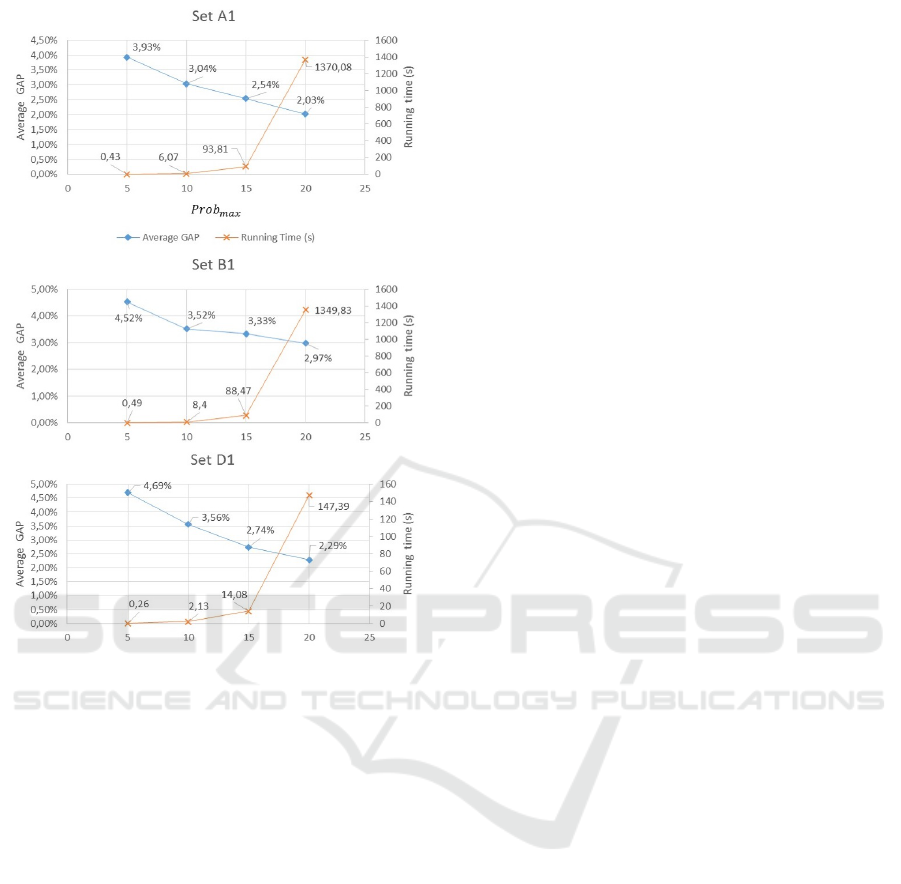
Figure 5: Time and gap evolution chart.

average gap.

If we analyze the results for the multi-pass ver-

sion, we observe a reduction of the average gap go-

ing from 7.45% to 5.89%. Again, the algorithm

seems to give better results when the proportion of

non-preemptive activities is high (Set C). There is

not enough statistical evidence to conclude about the

other instances sets.

For small instances (sets A, B, C and D), run-

ning time seems not to be a problem (even when we

use a high value for Prob

max

). However, for bigger

instances (sets A1, B1, C1 and D1), running time

may become prohibitive for high values of Prob

max

We wanted to study the behavior of the solving time

and the average gap when we increase the value of

Prob

max

. Using the multi-pass version of the local

search algorithm, we measure average time and gap

for different values of Prob

max

(5%, 10%, 15% and

20%) for those instances solved to optimality; these

values are presented in Figure 5. Results for Set C1

are not presented in Figure 5 since only 1 instance

was solved to optimality. However, for highly non-

preemptive activities solving time remains reasonable

(less than 15 sec) even when Prob

max

goes to 75%.

The curves in Figure 5 show similar behaviors for

highly preemptive (Set A1) and partially preemptive

(Set B1) instances. This was expected, since for these

two types of activities, we may re-evaluate the tech-

nicians allocations for every unit time of the activ-

ity duration (what increases signiﬁcantly the number

of nodes in the search tree). We observed an ex-

ponential increase on the average solving time when

Prob

max

= 20% for all sets of instances; this while the

average gap presents an exponential decrease. Also

as expected, the average time for solving instances

within Set D1, is lower than for instances within

sets A1 and B1; this is due to the presence of more

non-preemptive activities. If we take the results for

Prob

max

= 15% (the best compromise solving time

and average gap) as reference point, we observe an

important reduction of the general average gap de-

creasing from 4.98% (for the multi-pass version of the

greedy algorithm) to 2.88%.

5 CONCLUSIONS AND FUTURE

RESEARCH

In this article we consider a new variant of the Multi-

Skill Project Scheduling Problem including partial

preemption (MSPSP-PP). The main characteristics of

this variant is the innovative way we handle the re-

lease of resources during preemption periods. Instead

of releasing of resources, as we do in classical pre-

emptive scheduling, we will release only those hav-

ing a smal setup time/cost. The proposed problem can

be easily adapted to other ﬁeld, specially those where

setup times/costs are important or hard to estimate.

The MSPSP-PP is NP-hard, we then propose a

greedy algorithm based on priority rules and using

a serial schedule generation scheme. To solve the

subproblem of technicians allocation, we proposed to

model it as a Minimum-Cost Maximum-Flow prob-

lem. The proposed algorithm gives us encouraging

results that are improved when we used it as a multi-

pass heuristic, obtaining an average gap of 7.45%.

In order to improve the solution obtained with the

greedy algorithm, we proposed a randomized tree-

based local search algorithm that allows us to reduce

the average gap from 4.98% to 2.88%. Both algo-

rithms seem to give better results when the proportion

of non-preemptive activities is high.

As future work, we must study the way to choose

the right value for the probability of visiting the right-

hand branch in the search tree, in order to have a com-

promise between the solutions quality and the time

required to get them. A different approach for gener-

ating the tree search node is also necessary in order to

A Heuristic Method for the Multi-skill Project Scheduling Problem with Partial Preemption

119

Table 7: Gap for the tree-based local search algorithm.

Gap

All A B C D

Gap Improv. Gap Improv. Gap Improv. Gap Improv.t Gap Improv.

LD 8.86% 2.78% 10.18% 1.73% 8.91% 3.02% 6.66% 4.12% 9.70% 2.23%

MS 9.29% 2.02% 9.46% 2.40% 9.28% 2.59% 8.33% 1.01% 10.08% 2.08%

EST 9.92% 3.33% 9.92% 4.52% 10.71% 2.43% 9.11% 2.52% 10.68% 3.83%

EFT 10.11% 3.77% 10.11% 5.15% 10.53% 2.38% 13.76% 4.12% 10.13% 3.44%

GR 9.46% 2.48% 9.46% 2.40% 9.28% 2.59% 8.18% 2.85% 10.08% 2.08%

GRD 9.47% 3.01% 9.47% 3.81% 9.00% 2.83% 8.06% 3.60% 9.19% 1.81%

Multi-pass 5.89% 1.88% 5.89% 1.99% 6.10% 2.67% 4.14% 0.62% 5.69% 2.24%

improve the solving times.

Experimental tests show that the proposed heuris-

tic is very sensitive to the sequence (priority rule) we

use. We must then identify the structure of the opti-

mal sequences in order to improve our results.

REFERENCES

Ababei, C. (2009). C++ adapted version of the

Edmonds-Karp relabelling MCMF algorithm.

https://github.com/eigenpi/MCMF4. Online; ac-

cessed 01 September 2018.

Ahuja, R. K. (2017). Network Flows: Theory, Algorithms,

and Applications. Pearson Education, 1st edition.

Almeida, B. F., Correia, I., and Saldanha-da Gama, F.

(2016). Priority-based heuristics for the multi-skill re-

source constrained project scheduling problem. Ex-

pert Systems with Applications, 57:91–103.

Artigues, C. (2008). The resource-constrained project

scheduling problem. In Resource-constrained project

scheduling: models, algorithms, extensions and appli-

cations, pages 21–36. John Wiley & Sons.

Ballest

ın, F., Valls, V., and Quintanilla, S. (2008).

Pre-emption in resource-constrained project schedul-

ing. European Journal of Operational Research,

189(3):1136–1152.

Ballest

ın, F., Valls, V., and Quintanilla, S. (2009). Schedul-

ing projects with limited number of preemptions.

Computers & Operations Research, 36(11):2913–

2925.

Bellenguez-Morineau, O. (2008). Methods to solve multi-

skill project scheduling problem. 4OR, 6(1):85–88.

Correia, I. and Saldanha-da Gama, F. (2015). A modeling

framework for project stafﬁng and scheduling prob-

lems. In Schwindt, C. and Zimmermann, J., editors,

Handbook on Project Management and Scheduling

Vol.1, International Handbooks on Information Sys-

tems, pages 547–564. Springer International Publish-

ing, Cham.

Derrick, B., Toher, D., and White, P. (2017). How to com-

pare the means of two samples that include paired

observations and independent observations: A com-

panion to Derrick, Russ, Toher and White (2017).

Tutorials in Quantitative Methods for Psychology,

13(2):120.

Edmonds, J. and Karp, R. M. (1972). Theoretical improve-

ments in algorithmic efﬁciency for network ﬂow prob-

lems. Journal of the ACM (JACM), 19(2):248–264.

Harvey, W. D. and Ginsberg, M. L. (1995). Limited dis-

crepancy search. In International Joint Conferences

on Artiﬁcial Intelligence, pages 607–615.

eron, E. (2002). Lower bounds for the multi-skill project

scheduling problem. In Proceedings of the Eighth

International Workshop on Project Management and

Scheduling, Valencia, Spain.

Polo-Mej

ıa, O., Anselmet, M.-C., Artigues, C., and Lopez,

P. (2018). Mixed-integer and constraint programming

formulations for a multi-skill project scheduling prob-

lem with partial preemption. In 12th International

Conference on Modelling, Optimization and Simula-

tion (MOSIM 2018), 8 pages, Toulouse, France.

Sourd, F. (2001). Scheduling tasks on unrelated machines:

Large neighborhood improvement procedures. Jour-

nal of Heuristics, 7(6):519–531.

Vanhoucke, M. (2008). Setup times and fast tracking in

resource-constrained project scheduling. Computers

& Industrial Engineering, 54(4):1062–1070.

Voß, S., Fink, A., and Duin, C. (2005). Looking Ahead with

the Pilot Method. Annals of Operations Research,

136(1):285–302.

ICORES 2019 - 8th International Conference on Operations Research and Enterprise Systems

120