A State Dependent Chat System Model
Per Enqvist
1
and G
¨
oran Svensson
1,2
1
Division of Optimization and Systems Theory, Kungliga Tekniska H
¨
ogskolan, Lindstedtsv 25, Stockholm, Sweden
2
Teleopti WFM, Teleopti AB, Karlav
¨
agen 106, Stockholm, Sweden
Keywords:
Chat System, Queueing Network, Modeling.
Abstract:
The main purpose of this paper is to introduce a model of a chat based communication system, as well as
developing the necessary tools to enable resource optimization with regards to a measure of the service qual-
ity. The system is modeled by a Markov process in continuous time and with a countable state space. The
construction of the intensity matrix corresponding to this system is outlined and proofs of a stationary state
distribution and an efficient way of calculating it are introduced. A numerical example for system optimization
when the service measure is the average sojourn time is included as well as a heuristic algorithm for quicker
solution generation.
1 INTRODUCTION
In this paper a chat based communication system
model is developed and used. It is based on the patent
(Svensson, 2018). The type of service system in-
vestigated is a Markov process {X(t),t ∈ R
+
} on a
countable state-space X . The main difference from a
more traditional queueing system, such as a M/M/s-
queue, is that the service intensities are state depen-
dent. This state dependency is introduced to model
a server (agent) being able to work on several tasks
in parallel. In particular, such a system can model a
chat based communication system at a modern con-
tact center, which will be the focus of this paper.
However, the main ideas may just as easily be applied
to any similar phenomena. Here, this feature is mod-
eled by attributing variable service rates to servers
under different workloads. The number of jobs a
server is currently serving in parallel is called the con-
currency level. This setting shares many similarities
with the field of processor sharing, such as (Klein-
rock, 1967), (Cohen, 1979), and limited processor
sharing, see (Yamazaki and Sakasegawa, 1987), (Avi-
Itzhak and Halfin, 1989) and in particular it is similar
to limited and variable processor sharing (Rege and
Sengupta, 1985), (Gupta and Zhang, 2014). The key
difference lies in the fact that the amount of service
needed to complete a job is not known until it is fin-
ished, whereas in the processor sharing framework the
size of the job is known once it enters the system.
In Section 2 the state space based queueing model
is introduced, with focus on the intensity matrix, de-
noted by Q. In Section 3 the closed form solutions
for the problem are discussed, first for a single agent
handling several tasks in parallel and then for general
instances of modeled queueing system. In Section 4
several measures of Quality of Service (QoS) are dis-
cussed, relevant optimization formulations are intro-
duced and some numerical examples are given. For
the QoS measures the differences as compared with
similar measures for telephone systems are deliber-
ated on. These measures are intended to represent a
relevant indication of customer and provider satisfac-
tion. Many such measures may be devised, in this text
the focus will be on the the customer sojourn time.
Given a QoS measure and a minimum requirement
to be fullfilled the optimal number of concurrent cus-
tomers per agent and group can be determined, as well
as the optimal routing in terms of where to route an
arrival as well as setting the maximum concurrency
level for the agents.
2 SYSTEM MODEL
A queueing system, where the servers can work on
several tasks in parallel is modeled. Since this work
pertains to chat-based communication in a contact
center environment, the servers of classical queueing
systems may be referred to as agents and the arrivals
will be considered to be arriving customers or clients
in a chat queue, they will sometimes also be referred
Enqvist, P. and Svensson, G.
A State Dependent Chat System Model.
DOI: 10.5220/0007391001210132
In Proceedings of the 8th International Conference on Operations Research and Enterprise Systems (ICORES 2019), pages 121-132
ISBN: 978-989-758-352-0
Copyright
c
 2019 by SCITEPRESS – Science and Technology Publications, Lda. All rights reserved
121

to as tasks or jobs. Once an agent answers an open
chat, it is assumed to be the start of the service pe-
riod of that specific chat dialogue and the end of the
waiting time in queue for that customer. Any change
of state happens instantaneously. All state changes
(jump process) will be right-continuous with left lim-
its everywhere with probability one (c
`
adl
`
ag).
2.1 Model Components
Let {X(t);t ∈ R
+
} be a Markov process on a count-
able state space X , in continuous time t. The state
space is given by all possible combinations of job dis-
tributions over server groups and including a buffer
for waiting customers. Consider such a process when
the parameters allow a steady state solution, i.e., the
system is stable as limt → ∞. Then the transition
probabilities depend only on the current state, not on
time, and the state distribution is independent of ini-
tial conditions. Using the idea of a chat based system
where servers may work on several jobs in parallel
the underlying state space can be constructed, which
correspond to the number of jobs in the system and
their distributions over the available servers and the
buffer. The parameters determining the state space
and the transition rates include the number of servers
(or groups of servers if they are not exchangable),
the rate at which arrivals occur, the service rates un-
der different customer distributions and the routing of
customers to servers or server groups.
2.1.1 Arrivals
In the following all customer arrivals are considered
to be independent and identically distributed, further
it is assumed that all tasks are equal in the sense that
they are indistinguishable from one another in terms
of service required, i.e., there exist a single class of
customers. The arrival process is also assumed to be
independent of the service process.
The rate at which new arrivals enter the queueing
system is taken to follow a homogeneous Poisson pro-
cess with rate parameter λ. It is assumed that there is
one common buffer for all arriving customers, if there
are no service slots available.
2.1.2 Servers and Server Groups
All servers belong to some group, indexed by G =
{1,...,G}. Agents from the same group are ex-
changable. Let there be s
i
∈ N agents in group i ∈
G and let s = [s
1
s
2
... s
G
]
T
be the corresponding
staffing vector.
An agent can be idle or actively serving a number
of customers up to the maximum concurrency limit
n
i
,i ∈ G. Let n = [n
1
n
2
... n
G
]
T
represent the vector
of maximum limits of the number of jobs a server may
simultaneously work on. Then the maximum number
of customers that may be receiving service is given by
J
max
= n
T
s, i.e., the number of service slots.
The individual agent’s state will be defined by the
number of concurrently served customers.
Let Y
i
= {1,...,n
i
} denote the state space for a
typical agent of group i ∈ G, corresponding to the
number of customers being served. An agent’s state
may then be denoted by s
i
j
, corresponding to agent
j ∈ {1,2,. . . , s
i
} in group i ∈ G.
The state of group i at some time point t can be
captured by a state vector X
i
(t) ∈ N
n
i
+1
, which counts
the number of agents in each state for the group
X
i
(t) =
s
i
∑
j=1
n
i
∑
k=0
I(s
i
j
= k)e
k
, i ∈ G, (1)
where I denotes the indicator function and where e
k
is the unit vector in the direction of k ∈ Y
i
. Some ad-
ditional organizational structure may be imposed for
book keeping purposes when needed.
The service rate of an agent will depend on the
state of that agent, i.e., the number of customers being
served. The total service rate, pertaining to an agent,
is assumed to be split equally between the served cus-
tomers. The service times are assumed to be exponen-
tially distributed with intensity parameter µ
i
k
, which
depends on the group i ∈ G and the current state k ∈ Y
i
of the agent.
The total service rate when all agents are serving
their maximum number of customers will be denoted
by µ
tail
(n) =
∑
G
i=1
s
i
µ
i
n
i
. Depending on the choice of
n, µ
tail
will take different values. It is often fruitful
to set this value equal the maximum possible service
capacity.
Figure 1 depicts three agents, from the same
group, serving a varying number of clients. Note the
varying service rates. In general there is no need for
further restrictions on the agent’s service intensities,
however, it is reasonable to expect that the service
per customer is decreasing for increasing concurrency
levels.
Assumption 2.1 In this article it will be assumed that
the service intensity per customer, µ
i
k
/k, is a decreas-
ing function of the number of concurrent customers.
The total service rate, µ
i
k
, of an agent may increase as
more concurrency is allowed, see Figure 2. This as-
sumption implies that the total service rate of an agent
is an integer concave function in terms of the number
of clients being served.
ICORES 2019 - 8th International Conference on Operations Research and Enterprise Systems
122

Figure 1: System of three agents, where agents 1 and 3 serve
several customer simultaneously. Figure by Carl Rockman.
0 1 2 3 4 5 6 7 8 9
No. of Concurrent Jobs
0.2
0.4
0.6
0.8
1
1.2
1.4
Service Intensity
Total Service Intensity
Figure 2: Total service rate for a single server under differ-
ent number of concurrent customer loads.
2.1.3 Buffer
If an arriving customer can not be served immedi-
ately then the customer is placed on hold, waiting in
a buffer. The buffer may be infinite in size and is
following the queueing discipline of first come first
served (FCFS). A client waits in this queue until an
agent has a free slot. Once the service slots have been
filled there will be a waiting queue forming. The state
of the buffer is denoted by X
b
∈ {0, 1, . . . }.
2.1.4 Routing
The process of matching arrivals to servers is handled
by a state dependent routing rule A = {a
i
(x)}
G
i=1
for
x ∈ X . Since it is state dependent the stationary solu-
tion do not satisfy the insensitivity property, i.e., the
product form solution. The term a
i
(x) corresponds to
the probability that the next arrival will be routed to
group i given that the system is in state x, see Assump-
tion 2.2.
A provides the controls for the system when there
are available service slots while the rule needs to be
extended to include the routing when there are no
available service slots. Let R = A ∪ {r
b
}, where r
b
represents routing a new job to the buffer. Since the
servers in the same group are exchangeable it does not
matter which specific one is in which specific state, all
that is needed is the distribution of the servers of the
group over the states. If a customer gets routed to the
buffer then this routing will be followed by a second
routing to the first available agent.
The routing rule R includes only inter-group rout-
ing while the intra-group routing will be done by
sending a new arrival to an appropriate agent, which
under most service measures will be to the agent with
the lowest current workload by Assumption 2.1. If
there are several servers, within a group, with an equal
number of jobs the new arrival is distributed uni-
formly. The specific routing is dependent on which
QoS measures are under consideration.
An assignment rule could also be made to incor-
porate other factors, such as fair work distribution be-
tween agents, priorites of groups and more. The one
condition on the routing rule is that it preserves the
Markovian property of the system.
Let L : X → N be a counting measure that returns
the total number of clients in the system given the cur-
rent state.
Assumption 2.2 For each k ∈ {1,...,n
i
}, i ∈ G and
R as given above, satisfies
(i) r
b
,a
i
≥ 0 and r
b
+
G
∑
i=1
a
i
(x) = 1, for all x ∈ X ,
(ii) A = 0 (identically zero) and r
b
= 1 if and only if
L(x) ≥ J
max
,
(iii) r
b
∈ {0, 1}.
2.2 Matrix Formulation
Traditional queueing systems are derived from the
pure birth-death process. The assumptions in Section
2.1 gives rise to a different type of queueing system.
Defining a Markov process in terms of generator ma-
trices provides a compact means of formulating the
system model.
When all agents are fully occupied then new ar-
rivals end up waiting in the queueing buffer. This part
of the system behaves as a birth-death process with
an arrival intensity λ and the total service rate of µ
tail
.
The corresponding intensity matrix structure is tridi-
agonal.
Pooling agents with identical performance into
groups limits the size of the system. See Figure 3
A State Dependent Chat System Model
123

and 4 for examples. The figures highlights the advan-
tages of grouping agents, in terms of system size. It
is realistic to expect that agents are grouped in a con-
tact center, in terms of the service they can provide.
From the examples depicted in the figures it can be
seen that the given routing rule aims at distributing
new arrivals as evenly as possible. Clients leaving the
system may result in an uneven distribution by which
is meant that the total system service intensity is lower
than the maximum possible intensity for that number
of jobs.
0,0 0,1 0,2
1,0 1,1 1,2
2,0 2,1 2,2
5
...
λ
2
λ
2
µ
1
1
λ
µ
1
2
λ
λ
µ
2
1
µ
2
1
µ
1
1
λ
2
λ
2
µ
2
1
µ
1
2
λ
µ
2
2
λ
µ
1
1
µ
2
2
λ
µ
1
2
µ
2
2
λ
µ
tail
λ
µ
tail
Figure 3: Example of a system with G = 2, n
1
= n
2
= 2 and
s
1
= s
2
= 1 with assignments to the least used agent, and
uniformly distributed if there is a tie.
2.2.1 System Intensity Matrix
As mentioned, a compact way to describe the queue-
ing system is in the form of an intensity matrix Q and
the corresponding state probability vector ¯p, which
determines the stationary state probabilities. Any
continuous time Markov process with some regular-
ity condition on the initial distribution can be uniquely
related to an intensity matrix Q.
Definition 2.3 (Intensity Matrix) . A matrix Q =
(q
i j
)
1≤i, j≤M
for some system size M, possibly infinite,
is defined as an intensity matrix (infinitesimal gener-
ator) if it satisfies the following conditions:
(i) 0 ≤ −q
ii
for all i ∈ {1,...,M},
(ii) 0 ≤ q
i j
for all i, j ∈ {1, . . . , M} with i 6= j,
(iii)
M
∑
j=1
q
i j
= 0 for all i ∈ {1,...,M}.
Note that the inequality in (i) is strict here.
0,0 0,1 0,2
1,1 1,2
2,2
5
...
λ
µ
1
1
λ
µ
1
2
λ
2µ
1
1
λ
µ
1
1
µ
1
2
λ
2µ
1
2
λ
µ
tail
λ
µ
tail
Figure 4: Example of a system with G = 1,n
1
= 2 and s
1
=
2 with assignments to the least used agent, and uniformly
distributed if there is a tie.
The intensity matrix governs the rate of state
changes of the Markov process X(t). The state of the
Markov system at any given time t is determined by
X(t) =




X
1
.
.
.
X
G
X
b




(t). (2)
Only one state change may occur at any given
time. There are four such possible types of changes
that may occur:
(i) An arrival occurs and is routed to an available
agent,
(ii) An arrival occurs and is routed to the buffer,
(iii) A departure occurs and a service slot becomes
available,
(iv) A departure occurs and the buffer is decreased.
All state changes occur on group level to keep the nu-
merical size to a minimum. For case (i) and (iii) a
change of state can then be handled on group level by
letting e
k
be a unit vector in the direction of k ∈ R
n
i
+1
and using this to update the system state on group
level. By assuming that at most one server in the
whole network transitions at any given time, the group
specific transition from state x ∈ Y
i
to y ∈ Y
i
may be
denoted by x
i
7→ x
i
+ (e
y
− e
x
). This corresponds to
a unique state change of the Markov process X(t) on
X .
In case (ii), i.e., that all servers are occupied when
a new arrival occurs then the routing sends the arrival
ICORES 2019 - 8th International Conference on Operations Research and Enterprise Systems
124

to the buffer which changes states accordingly X
b
7→
X
b
+ 1.
If there is a departure when the buffer is not empty,
case (iv), then the buffer changes as X
b
7→ X
b
− 1
and the state of the corresponding group remains un-
changed as x
i
7→ x
i
+ (e
x
− e
x
).
The current state of the system is given by X(t),
which is fully determined by the distribution of jobs
between the different groups and the buffer. Each
state is represented by a row in the intensity matrix
Q.
When an arrival occurs it does so with an inten-
sity of λ and if there is at least one service slot free
then it gets routed to an available agent, which corre-
sponds to a thinned state dependent Poisson process.
When there are no free service slots the new arrival
gets routed to the buffer. The intensities with which
the arrivals are routed to the different groups, or the
buffer, are given by
(
λ
i
(x) = a
i
(x)λ, x ∈ X
1:J
max
,
λ
i
(x) = r
b
λ, x ∈ X
(J
max
+1):M
,
for all i, (3)
where X
1:J
max
correspond to there being at least one
service slot free to recieve an arriving client and
X
(J
max
+1):M
when there are no available servers.
On the other hand departures leave the system
from group i in state X
i
(t) with intensity
µ
i
(x) = [µ
i
0
µ
i
1
... µ
i
n
i
]X
i
(t), i ∈ G. (4)
Definition 2.4 (System Intensity Matrix) . Let Q be
the intensity matrix corresponding to the Markov pro-
cess X (t), satisfying Definition 2.3 and with jump in-
tensities given by Equations (3) and (4). The states
for which X
b
= 0 are first in order followed by the
states for which X
b
> 0, in ascending order of the
total number of clients in the system. Furthermore,
let the first row correspond to the empty system state
and the (J
max
+ 1):th row be the state for which all
service slots are filled but the buffer is empty. Let
N = J
max
+ 1.
This intensity matrix can be partitioned into four
submatrices, as shown in Equation (5). This parti-
tion will make further analysis of the system more
tractable.
Q =

A B
C D

(5)
The first submatrix, A, correspond to states for
which the buffer is empty, see Definition 2.4. It is
a sparse band matrix of size N × N. The size becomes
considerably smaller if the servers are grouped into a
few groups.
The two submatrices B and C may both be infinite
but contain only one non-zero element each.
B =



0 0 ···
.
.
.
.
.
.
···
λ 0 ···



, (6)
C =



0 ··· 0 µ
tail
0 ··· 0 0
.
.
.
.
.
.
.
.
.
.
.
.



. (7)
The fourth submatrix, D, corresponds to the states
for which there is a queue. The intensity submatrix
D has the expected tridiagonal form of a traditional
M/M/· system, i.e., it corresponds to a standard birth-
death process and may be infinite in size.
D =




d λ 0 0 · ··
µ
tail
d λ 0 · ··
0 µ
tail
d λ ···
.
.
.
.
.
.
.
.
.
.
.
.




, (8)
where d = −(λ + µ
tail
) except for the last row where
it is −µ
tail
.
2.3 System Structure
The use of the intensity matrix, given by Equation
(5), requires that the system matrix can be created
for different numbers of groupings of agents and dif-
ferent maxima on concurrency levels. The structure
of the submatrices B,C and D are given in (6) - (8).
It is only the system size that varies the structure of
those submatrices. The construction of A is given by
Equations 3 and 4. The matrix A depends on a given
assignment rule, A, which determines the routing of
new arrivals within the system. The submatrix A is of
finite size for all realistic systems, it might however be
of interest to study its behaviour under different lim-
iting schemes, compare with the Halfin-Whitt heavy
traffic regime (Whitt and Halfin, 1981).
In the empty system, corresponding to the first
row of Q, only arrivals may occur. The exact order
of the rows is important when implementing a numer-
ical model of the system, but here it suffices that the
first and last row of A are clearly defined.
Example: For some ordering of the states the in-
tensity matrix for Figure 3 has the following structure
A State Dependent Chat System Model
125




















d
1
λ
2
0
λ
2
0 0 0 0 0 0 0 ···
µ
1
1
d
2
0 0 λ 0 0 0 0 0 0 ···
0 µ
1
2
d
3
0 0 λ 0 0 0 0 0 ···
µ
2
1
0 0 d
4
λ 0 0 0 0 0 0 ···
0 µ
2
1
0 µ
1
1
d
5
λ
2
0
λ
2
0 0 0 ···
0 0 µ
2
1
0 µ
1
2
d
6
0 0 λ 0 0 · · ·
0 0 0 µ
2
2
0 0 d
7
λ 0 0 0 ···
0 0 0 0 µ
2
2
0 µ
1
1
d
8
λ 0 0 · · ·
0 0 0 0 0 µ
2
2
0 µ
1
2
d
9
λ 0 ···
0 0 0 0 0 0 0 0 µ
tail
d
10
λ · · ·
.
.
.
.
.
.
.
.
.
.
.
.
.
.
.
.
.
.
.
.
.
.
.
.
.
.
.
.
.
.
.
.
.
.
.
.
,



















where the d
i
:s are the negative sum of the off-diagonal
row elements.
The routing rule will be determined in relation to
one or more QoS measures, see Section 4. Different
measures may imply different routing rules, e.g., un-
der some circumstances minimizing the average wait-
ing time in the system and the average waiting time in
the buffer produces different routing and even differ-
ent concurrency levels for the servers.
3 STATE PROBABILITY
DISTRIBUTION
An important goal of modeling a system in steady
state is to determine if there exists a stationary state
distribution, ¯p, and the necessary conditions associ-
ated with it. The solutions to this question will be
answered first for a single agent and then for a system
of multiple agents and groups.
3.1 Single Agent, Multiple Tasks
Queueing System
Looking at a queueing system with a single agent that
can serve up to n customers concurrently. Assum-
ing that the system is in steady state and of the type
M/M/n. It is also assumed that the service rate per
customer is a nonincreasing function of the number
being served and that the service amount is evenly dis-
tributed amongst the clients. Since only one agent is
considered the group index may be dropped.
Introduce the state probabilities p
i
for i = 0,1,....
The arrivals are assumed to follow a time homoge-
neous Poisson process with intensity parameter λ.
Only one class of customers is considered. The fol-
lowing expressions will be used in determining the
state probability distribution for the given queueing
system in equilibrium
ρ
i
=
(
i
λ
µ
i
, i ≤ n
n
λ
µ
n
, i > n,
(9)
where µ
i
is the total service intensity for state i ≤ n
and µ
n
for i > n when there are i tasks in the queue.
Let
ρ(i) =

∏
i
j=1
ρ
j
if i ≤ n
ρ
i−n
n
∏
n
j=1
ρ
j
if i > n.
(10)
The load, ρ(i), depends on the number of total tasks
in the system, both tasks that are being served and
those in the buffer . To achieve steady state the system
must be either finite or
λ
µ
n
=
1
n
ρ
n
< 1 must hold if the
buffer size is infinite. The probability of each state
can be expressed in terms of the empty system state
probability, p
0
, via the local or global flow balance
equations
p
i
=
(
1
i!
ρ(i)p
0
if i ≤ n

1
n

i−n
1
n!
ρ(i)p
0
if i > n.
(11)
From Markov theory it is well known that for a birth-
death process where λ/µ
n
< 1 there exist a stationary
distribution. Since
∑
∞
i=0
p
i
is a sum of probabilities,
when the steady state condition holds, there is a so-
lution for p
0
determined by the following expression
for p
0
p
0
= 1 +
n−1
∑
i=1
1
i!
ρ(i) +
ρ(n)
n!
n
n − ρ
n
!
−1
. (12)
Since λ and the µ
i
:s are known we can calculate p
0
and hence also p
i
, for any i ∈ N.
3.2 Multiple Agents and Multiple Tasks
Queueing System
Consider the situation where there are several agents
handling incoming tasks. These agents may be
grouped into pools with other agents with whom they
are exchangeable. We will look at the case where
there is only one class of jobs. The state probabilities
will be calculated for the potentially infinite queueing
system.
To solve the complete system described in Sec-
tion 2 a few preliminary results will have to be shown.
A stationary distribution ¯p can be found when
µ
tail
> λ holds. It is shown that there exist a limiting
distribution, which is equivalent to the stationary state
distribution, by means of finding the unique solution.
Use the partitioning of the intensity matrix Q from
Equation (5). Suppose that Q ∈ R
M×M
, A ∈ R
N×N
ICORES 2019 - 8th International Conference on Operations Research and Enterprise Systems
126

where N = J
max
+ 1 and that M ≥ N. The steady state
solution for the Markov system then satisfies
x Q = 0. (13)
It is helpful to partition the state vector into two parts,
matching the partition in (5) so that x = (x
1
x
2
), where
x
1
∈ R
N
and x
2
∈ R
M−N
. Then Equation (13) can be
stated as
(x
1
x
2
)

A B
C D

= (0 0). (14)
Since D is invertible due to tridiagonal birth-death
structure, the following holds
(
x
1
A + x
2
C = 0
x
1
B + x
2
D = 0
=⇒
(
x
2
= −x
1
BD
−1
x
1
(A − BD
−1
C) = 0.
(15)
Remark 3.1. The first Equation in (15) indicates that
the probabilites of the states of the x
2
-vector only de-
pend on the last element of the x
1
-vector since subma-
trix B only contains one nonzero element, in the last
row of the first column.
That the constructed intensity matrix Q is irre-
ducible will be used repeatedly, thus, it is prudent to
show that this is indeed the case.
Lemma 3.2. The system matrix Q is irreducible if N
is finite.
Proof. When all service slots are filled, L(X(t)) ≥ N,
the process has a pure birth-death structure and thus
this part is irreducible and communicating with the
system state L(X(t)) = N.
For the situation when L(X (t)) ≤ N, the irre-
ducibility may be shown state by state. By con-
struction no state is absorbing, the arrival and ser-
vice intensities are finite and λ, µ
i
k
> 0. The state
L(X(t)) = 0 and L(X(t)) = N communicate since
all accepted routing rules route new arrivals to some
system state with one more job in the system with
positive probability and any distribution of occupied
servers can always reach L(X(t)) = 0 since all ser-
vice rates are positive. Thus all intermediate states
between L(X(t)) = 0 and L(X(t)) = N are reachable,
with positive probability, from L(X (t)) = N. Thus
since any configuration can reach the empty system
state and this state communicates with L(X(t)) = N
which in turn communicates with all states for which
L(X(t)) > N the whole chain of Q is irreducible.
To solve the system it is useful to first show that
the A matrix has full rank for all systems where the
size of the intensity matrix Q is at least of size N +
1 × N + 1. Let the N × N matrix
˜
A be
˜
A =
(
A, M = N,
A + λe
N
e
T
N
, M ≥ N + 1,
(16)
where e
N
is a unit vector in the N:th direction and
where the intensity matrix Q has been ordered such
that the N:th row corresponds to the state for which
all agents are fully occupied but the buffer is empty
and where the states following the N:th state are or-
dered in terms of increasing number of customers in
the system.
Remark 3.3. For an irreducible intensity matrix Q ∈
R
M×M
, where M ≥ N, it holds that rank(
˜
A) = N − 1,
since it represents a finite irreducible Markov chain.
Lemma 3.4. For an irreducible Markov system de-
fined by the intensity matrix Q of Section 2.2.1, with
Q ∈ R
M×M
and where M ≥ N + 1 it holds that the
submatrix A of Q has rank N.
Proof. Let Q be the following intensity matrix
Q =

A b
c
T
d

, (17)
where b ∈ R
N
, c
T
∈ R
N
and d ∈ R. Then Q ∈
R
(N+1)×(N+1)
represents an irreducible Markov sys-
tem. By construction, Q1 = 0, the final column of Q
can be expressed as a linear combination of the other
columns

b
d

= −
∑
i

A
c
T

i
. (18)
Then the submatrix (A c
T
)
T
in (17) has at most N in-
dependent columns. It remains to show that c
T
is a
linear combination of the rows of A. The sub matrix
(A c
T
)
T
also has N independent rows and it suffices to
show that c
T
is a linear combination of the rows in A.
To do that turn to the matrix
˜
A, which by construction
has rank(
˜
A) = N −1, since it is an intensity matrix for
a finite irreducible Markov system. Then there exists
a vector x
∗
∈ R
N
such that x
∗
> 0 and (x
∗
)
T
˜
A = 0.
The question becomes if there is a γ 6= 0 that satisfies
((x
∗
)
T
γ)

A
c
T

= (x
∗
)
T
A + γc
T
= 0, (19)
where c
T
= e
T
N
µ
tail
. Using
˜
A from Equation (16) to
obtain
0 = (x
∗
)
T
˜
A = (x
∗
)
T
(A + λe
N
e
T
N
)
= (x
∗
)
T
A + λ(x
∗
)
T
e
N
e
T
N
. (20)
By choosing γ =
λ(x
∗
)
T
e
N
µ
tail
=
λ(x
∗
)
N
µ
tail
6= 0 a nontrivial
solution to Equation (19) is found and hence c
T
can
be written as a linear combination of the rows of A
which in turn implies that rank(A) = N, i.e., A has
full rank.
A State Dependent Chat System Model
127

From the structure of B,C and D the following
holds
BD
−1
C =



0 ... 0
.
.
.
.
.
.
.
.
.
0 ... y
∗



= y
∗
e
N
e
T
N
(21)
for some scalar y
∗
and
ˆ
A = A − BD
−1
C = A −y
∗
e
N
e
T
N
,
where
ˆ
A = A − BD
−1
C is the Schur complement of Q.
Since x
1
(A−BD
−1
C) = 0 according to Equation (15),
the characteristic equation becomes
X
ˆ
A
(y) = det(A − y
∗
e
n
e
T
n
) = 0. (22)
Furthermore since the characteristic equation can
be expressed as X
ˆ
A
(y) = ay + b = 0 and X
ˆ
A
(y = 0) 6=
0 from Lemma 3.4 there exist a unique generalized
eigenvalue y. The unique value y
∗
= −λ gives that
ˆ
A =
˜
A.
The goal is to find the limiting distribution for the
system in steady state and to confirm that this is in-
deed equal to the stationary distribution ¯p. As before,
let the first N states correspond to the states for which
the buffer is empty, X
b
= 0. Partition the distribution
vector into two parts as done previously, x = (x
1
x
2
),
where x
1
corresponds to the states L(X (t)) ≤ N and
x
2
the states for which L(X(t)) > N. From general
theory of Markov systems it is known that the solu-
tion for an irreducible system in steady state can be
obtained by using the M − 1 independent equations
from the intensity matrix and augmenting the system
by use of the fact that the state vector is a probability
distribution, i.e. x adds to one,
∑
i
(x)
i
= 1, to obtain
a solution for the unique stationary state probability
distribution ¯p.
It will be shown that it is sufficient to solve
for a smaller problem in terms of the first N equa-
tions, which are independent since rank(A) = N from
Lemma 3.4. The solution is obtained by using x
1
˜
A =
0, from Equation (16), and the fact that the rest of the
state probabilities only depend on (x
1
)
N
i.e., the last
element of the x
1
-vector. Let
Q
I
=



1 | |
.
.
. q
2
... q
M
1 | |



(23)
˜
A
I
=



1 | |
.
.
. ˜a
2
... ˜a
N
ψ | |



(24)
where ψ =
∑
M−N
i=0

λ
µ
tail

i
and where the ˜a
i
represent
column i of the
˜
A matrix.
Proposition 3.5. Suppose that Q is the intensity ma-
trix for an irreducible Markovian system, as given in
Section 2.2.1, in steady state and Equations (23)-(24)
holds, then solving
(x
1
x
2
) Q
I
= (1 0 . . . 0) (25)
is equivalent to solving
x
1
˜
A
I
= (1 0 . . . 0) (26)
and calculating the state probabilities in x
2
as (x
2
)
i
=
(x
1
)
N

λ
µ
tail

i
for i = 1, 2, ..., M − N, where (x
1
)
N
rep-
resents the last element of the x
1
-vector.
Proof. Since x := (x
1
x
2
) is a probability distribution
it holds that
x
1
1
N
+ x
2
1
M−N
= 1. (27)
where 1
i
is a vector of i ones. Due to construction of
the intensity matrix and the local flow balance equa-
tions it also holds that
(x)
j+1
=
(
λ
µ
tail
(x)
N
=
λ
µ
tail
(x
1
)
N
, for j = N,
λ
µ
tail
(x)
j
=
λ
µ
tail
(x
2
)
j−N
, for j ≥ N +1.
(28)
Using ψ and Equations (27) and (28) together gives
1 = x
1
1
N
+ x
2
1
M−N
= (x
1
)
1:N−1
1
N−1
+ (x
1
)
N
+
M−N
∑
i=1

λ
µ
tail

i
(x
1
)
N
= (x
1
)
1:N−1
1
N
+ (x
1
)
N
ψ. (29)
This result is used in calculating the matrix multipli-
cation of the first column of the intensity matrix.
xQ
I
=(x
1
x
2
)










1 | |
.
.
. a
2
... a
N
B
1 | |
1 | |
.
.
. c
2
... c
N
D
1 | |










= (1 0 ... 0)
(30)
(x
1
x
2
)










1 | |
.
.
. a
2
... a
N
B
ψ | |
0 | |
.
.
. c
2
... c
N
D
0 | |










= [1 0 ... 0].
(31)
Solving Equation (31) in terms of x
1
, using the result
from Equation (15) results in
x
1










1 | |
.
.
. a
2
.. . a
N
ψ | |





− BD
−1
C





= x
1
˜
A
I
= (1 0 . . .0), (32)
where BD
−1
C is given by Equation (22), with y
∗
=
−λ.
ICORES 2019 - 8th International Conference on Operations Research and Enterprise Systems
128

Corollary 3.6. If M → ∞ then ψ →
µ
tail
µ
tail
−λ
and
lim
M→∞
x = ¯p.
Proof. By the definition of ψ and for a fixed value of
N, i.e., the size of A, which is constant for a given
system, ψ is given by
ψ = lim
M→∞
M
∑
i=N

λ
µ
tail

(i−N)
=
µ
tail
µ
tail
− λ
. (33)
Using results for a geometric series in Equation (33).
This being the unique solution to Equation (30), thus,
it is also the stationary state solution.
This method partitions the system in two, where
the second part may be handled as a pure birth-death
process with corresponding probability structure. For
a deeper study of such phenomena see (Boucherie,
1993).
Remark 3.7. The size of the generator matrix be-
comes very large even for moderate sized systems.
The advantage of using a small number of groups
play a significant role in keeping the size of the sys-
tem managable as does the employment of sparse nu-
merical methods. The intensity matrix Q is a sparse
matrix. The level of sparsity increases if the routing is
deterministic.
4 OPTIMAL NUMBER OF
CONCURRENT SERVICES PER
AGENT AND SERVICE LEVEL
In the previous sections a model describing a system
of grouped indistinguishable agents, able to handle
several tasks simultaneously at varying service rates,
has been introduced. One important question is how
to choose the planned level of maximum concurrency,
such that the system is optimal with respect to some
QoS measure/s. Another is how to choose the number
of servers to employ in each group. To answer these
questions one or more measures of QoS has to be de-
cided upon. There are many choices for such mea-
sures, see for example (Gans et al., 2003). Once the
measure, or measures, have been choosen, the perfor-
mance of the system w.r.t. that measure can be deter-
mined and optimized. The optimization process may
be performed iteratively, but to keep the amount of
calculations down a heuristic method for estimating
this number will be given below, with respect to the
average sojourn time for a customer.
4.1 Quality of Service Measures
Finding a model that fits the underlying system is of-
ten but a stepping stone in the process of managing a
queueing network. To evaluate different system con-
figurations some metric is needed. In service systems
the metric is commonly referred to as a Quality of Ser-
vice measure.
When looking at some of the measures used in tra-
ditional call centers it becomes apparent that some
modifications are in order. Two common measures
are Average Speed of Answer (ASA) and Traffic Ser-
vice Factor (TSF), where the first is given as the ex-
pected value of the amount of time the client has to
wait on service to begin, i.e., the call is answered
and the second one gives the fraction of clients that
start their service within a given time. For a chat sys-
tem, as described above, both these time measures
can be made zero by opening an infinite number of
service slots. However, the service rate per customer
would most likely be appaling. This suggests that the
QoS measure used should include aspects of the time
spent actually recieving service as well as the waiting
time. Some simple such measures might be the av-
erage head count process, i.e., the number of clients
in the system at a given time t or equivalently the ex-
pected sojourn time. If used sensibly the mean wait-
ing time in queue can successfully be used as the mea-
sure. It is worth noting that some routing rules and
system configurations may lead to shorter queueing
times while increasing the mean sojourn time, e.g.,
letting the agent concurrency level surpass the one
providing maximum total service rate may shorten the
waiting queue at the expense of longer sojourn times.
Definition 4.1. The sojourn time of a client is defined
as the time a customer spends in the system, from ar-
rival to the system until the departure from the system.
Let W ∈ R
+
be a random varible denoting the sojourn
time then the expected sojourn time is
EW = E(W ). (34)
Using the minimum average sojourn time for a
customer has the advantages of being fairly easy to
handle and Little’s law may be applied. For an indi-
vidual customer it might however be less favourable
since waiting times may be long for some customers,
the tail events. A drawback of using the mean sojourn
time measure is that it can be difficult to calibrate. In
the event that another measure is preferred the mini-
mum average sojourn time measure can still be used
as a initial value of an iterative search process.
In the general case both the maximum concur-
rency level and the number of agents per group con-
stitutes the targets but for the mean sojourn time the
A State Dependent Chat System Model
129

maximum concurrency level for minimizing the aver-
age number of clients in the system is just the con-
currency level where the total service rate is maxi-
mized. This follows from the fact that at each number
of clients in the system, L(X(t)), the rate at which
service is performed for the system is equal or higher
than for any other choice of n while the arrival rate is
the same. Thus, for the sojourn time measure it suf-
fices to find the optimal number and distribution of
servers over the groups. This translates to an assign-
ment rule that routes new clients as evenly as possible
if the total service rate is an integer concave function
of the concurrency level.
A special case is when there is only one group
with a linear increase in total service rate as a func-
tion of the concurrency level. Such a system may be
represented by a M/M/sn queueing system.
Another type of service measure that might be
worth considering is a fairness one, such as that the
time spent idling should be fairly evenly distributed
between groups and agents. In the example of Sec-
tion 4.3 below it will be shown why this would be an
interesting metric.
4.2 Optimization Formulation
Given the QoS measure, estimates of the system pa-
rameters and the costs of agents the problem may be
formulated as an optimimization problem. It is also
assumed that forecasts concerning the arrival process
are available. There are two main perspectives on
the optimization problem, the first being how many
agents are enough to fullfill demands of the service
quality as captured by the QoS measure,
(P)



min
s
∑
i
C
i
(s)
subj. to QoS(s,n) ≤ b
s,n ∈ Z
+



, (35)
and the second being given a budget how to best staff
the chat system to provide the best possible service.
The second formulation is mostly of interest when the
budget does not allow for sufficient staff to actually
fullfill the QoS level requirements.
(B)



min
s
QoS(s,n)
subj. to
∑
i
C
i
(s) ≤ B
s,n ∈ Z
+



, (36)
C is the agent cost function, b the required service
level and B is a budget constraint. It is assumed that
agents from the same group cost the same.
The optimization formulations may easily be re-
formulated to include multiple QoS measures and re-
strictions on agent availability.
4.3 Numerical Example
For a system that is measured on minimizing the aver-
age number of clients both the expected sojourn time
and the expected queueing time may be used as mea-
sures. In many cases it is easier to work with the time
a customer has to wait in line rather than the sojourn
time, since the average queueing time can be pushed
close to zero, while the sojourn time will depend on
the arrival rate and the single customer service rates.
When solving these types of problems it is possi-
ble to find the optimal solution via an iterative com-
binatorial approach, however, such a method is very
costly in terms of the number of calculations needed.
This really becomes an issue when dealing with large
systems, with a high degree of concurrency and many
groups. Even efficient and sparse solvers will struggle
to deliver solutions quickly. Thus, a simple heuristic
may be employed to achieve near optimal solutions
for realistic parameters. Given some starting distri-
bution of agents over the groups such that, s
i
j
> 0,
for all i ∈ G and j ∈ {1, . . . , s
i
}, then one agent at
a time is added according to some prediction func-
tion κ(s) : N
G
→ G. This function calculates marginal
gains for each group in terms of service rate per cost
of agent, and then returns the corresponding group in-
dex with the largest marginal gain. The service rate
used is based on a prediction of what state an addi-
tional agent would be in and uses the corresponding
service rate.
To decide which group receives the additional
agent the heuristic looks at the current system so-
lution and determines the most likely (weighted fre-
quency) concurrency level of each group. These lev-
els are used to calculate the corresponding marginal
gains,
µ
i
k
C
i
, to compare the benefits of adding agents to
the different groups and picks the one with the largest
marginal gain. In the next step the system is solved
with the predicted agent distribution and if the new so-
lution predicts another agent to be added to the same
group then the choice is accepted. However, if the
new solution indicates that a new group is to receive
an additional agent then all possible updates are com-
pared and the QoS measures determine the best up-
date. The drawback of using this heuristic is that there
are situations where the algorithm reacts too slowly,
as can be seen in the example below.
In general the heuristic will provide means to con-
trol a base distribution of agents between groups,
which may be dictated by contracts, etc. It will also
generate near optimal solutions at a much lower com-
putational cost than the combinatorial approach. It
works best when the service level of the groups dom-
inate each other consistently. Near efficient points are
ICORES 2019 - 8th International Conference on Operations Research and Enterprise Systems
130

Algorithm 1: Starting with a staffing vector such that
QoS(s) is defined, heuristically determine a new staffing
vector such that QoS(s) ≤ b.
Data: G,s,n,λ,µ
i
k
:s, b
initialize ;
s
i
> 0 ∀i ∈ G ;
solve system and calculate QoS(s) ;
while QoS(s) > b do
compute k = κ(s) ;
let s
tmp
→ s + e
k
;
solve system for s
tmp
;
compute k
tmp
= κ(s
tmp
) ;
if k equals k
tmp
then
s → s
tmp
;
else
for i=1:G do
solve system for s → s + e
i
end
choose s s.t.
QoS(s) = min
i=1:G
QoS(s + e
i
) ;
end
end
calculated as a side effect of the heuristic, which may
be used to solve either (35) or (36).
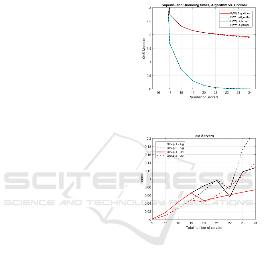
Example
In this example the expected sojourn times, the
expected waiting times and the idleness of average
agents of group 1 and 2, respectively, have been in-
vestigated. The solutions are in terms of the ex-
pected sojourn times. The parameters used are as fol-
lows G = 2,n
1
= n
2
= 2 and both groups start with
s
1
= s
2
= 8 agents each. Servers from the first group
are more efficient than members of the second group
when working with a single customer while the agents
of group two have higher service rates for two concur-
rent clients. The arrival rate is given by λ = 13.5 and
the service rates are µ
1
0
= 0,µ
1
1
= 0.6,µ
1
2
= 0.8,µ
2
0
=
0,µ
2
1
= 0.5, µ
2
2
= 0.9 and both types of agents have
C = 1. The servers in Figure 5 will have a de-
creasing workload as more servers are added, with a
jump when the system changes from adding servers
to group two to group one, which can be seen in Fig-
ure 6. The complete set of values may be viewed in
Table 1 and 2.
The example was chosen such that the heuristic
would perform suboptimally. It seems the solution,
both the optimal and the heuristic, behaves in ac-
cordance with the ”law of diminishing returns” (see
(Koole and Pot, 2011) for a discussion), i.e., the QoS
measure is integer convex in the number of servers.
Furthermore, it can be noted that although the optimal
Figure 5: The expected sojourn times and the expected
queueing times for the optimal solution as compared to the
algorithm. Where E(W) is the expected sojourn time and
E(Wq) the time waiting in the queue.
Figure 6: The percentage of the time agents from group 1
and 2 are idle for the algorithm solution and the optimal
solution.
Table 1: The algorithm solution generated.
Qos Idleness Numbers
Agents E(W) E(W
q
) grp1 grp2 grp1 grp2
16 11.7223 11.5862 0.0016 0.0009 8 8
17 2.7588 1.6885 0.0170 0.0099 8 9
18 2.3078 0.7150 0.0430 0.0276 8 10
19 2.1526 0.3037 0.0653 0.0480 8 11
20 2.0746 0.1214 0.0831 0.0715 8 12
21 2.0278 0.0450 0.0962 0.0981 8 13
22 1.9856 0.0158 0.0563 0.0748 9 13
23 1.9494 0.0051 0.1177 0.1725 10 13
24 1.9177 0.0015 0.1276 0.2228 11 13
solution generates solutions with lower sojourn times
the waiting times in queue are lower for the heuris-
tic solution which illustrates the point made in Sec-
tion 4.1. The intuition is that the waiting times are
more dependent on the total service provided when
the concurrency level is maximized.
A State Dependent Chat System Model
131

Table 2: The optimal solution generated.
Qos Idleness Numbers
Agents E(W) E(W
q
) grp1 grp2 grp1 grp2
16 11.7223 11.5862 0.0016 0.0009 8 8
17 2.7588 1.6885 0.0170 0.0099 8 9
18 2.3078 0.7150 0.0430 0.0276 8 10
19 2.1526 0.3037 0.0653 0.0480 8 11
20 2.0718 0.1276 0.0462 0.0429 9 11
21 2.0132 0.0489 0.0539 0.0601 10 11
22 1.9664 0.0170 0.0608 0.0815 11 11
23 1.9271 0.0054 0.0672 0.1079 12 11
24 1.8934 0.0016 0.0733 0.1396 13 11
Looking at Figure 6 it can be seen that the work
distribution between the groups, in terms of time
spent in the idle state, is quite uneven. Thus a fair-
ness measure might be relevant to mitigate some of
that effect.
5 SUMMARY AND
CONCLUSIONS
We have shown how a queueing system, where
the servers handle several tasks simultaneously and
where the total service rate for a server varies with
the number of concurrent jobs handled, can be con-
structed. The construction is general under the im-
posed conditions of the system being in steady state,
irreducible and Markovian. It can be constructed in
such a way that each agent is considered to be its own
group, which means that the impact of each agent on
the system can be measured and estimated. However
the number of system states will increase very quickly
which in practice will limit the number of groups that
can be considered. Also it would, in most cases, be
hard to find sufficient data to estimate each agent sep-
arately to any degree of precision. This system can
be controlled in two ways, by assigning agents and by
means of the routing rules.
It is shown that it is sufficient to solve a smaller
system of linear equations than the whole system, to
calculate the steady state probabilities. The size of
this smaller system is R
N×N
. Once this smaller sys-
tem has been solved, the rest of the state probabilities
can be calculated recursively by a given formula.
By introducing a measure of the quality of service
we can say something about how the system performs
under different conditions. By using the average sys-
tem time for a customer as the measure of QoS, it is
shown how the optimal choice of maximum number
of simultaneous tasks should be chosen to minimize
average customer sojourn time. The solution is com-
pared to a heuristic method which is found to provide
results close to the true optimum.
A brief comparison between QoS measures of tra-
ditional call centers and that of chat systems is in-
cluded where the conclusion is that traditional mea-
sures must be handled sensibly or poor system per-
formance may result.
REFERENCES
Avi-Itzhak, B. and Halfin, S. (1989). Response times
in gated m/g/1 queues: The processor-sharing case.
Queueing Systems, 4(3):263–279.
Boucherie, R. J. (1993). Aggregation of markov
chains. Stochastic Processes and their Applications,
45(1):95–114.
Cohen, J. (1979). The multiple phase service network
with generalized processor sharing. Acta Informatica,
12(3):245–284.
Gans, N., Koole, G., and Mandelbaum, A. (2003). Tele-
phone call centers: Tutorial, review, and research
prospects. Manufacturing Service Oper. Management.
Gupta, V. and Zhang, J. (2014). Approximations and op-
timal control for state-dependent limited processor
sharing queues.
Kleinrock, L. (1967). Time-shared systems: a theoretical
treatment. Journal of the ACM (JACM), 14(2):242–
261.
Koole, G. and Pot, A. (2011). A note on profi
t maximization and monotonicity for inbound call
centers. Operations Research, (59(5)):1304–1308.
Rege, K. M. and Sengupta, B. (1985). Sojourn time distri-
bution in a multiprogrammed computer system. AT&T
Technical Journal, 64(5):1077–1090.
Svensson, G. (2018). Product and computer system for a
chat based communication system. US 10009468 B1,
USA.
Whitt, W. and Halfin, S. (1981). Heavy-traffic limits for
queues with many exponential servers. Operations
Research, 29(3):567–588.
Yamazaki, G. and Sakasegawa, H. (1987). An optimal de-
sign problem for limited processor sharing systems.
Management Science, 33(8):1010–1019.
ICORES 2019 - 8th International Conference on Operations Research and Enterprise Systems
132