GPU Accelerated Sparse Representation of Light Fields

Gabriel Baravdish, Ehsan Miandji and Jonas Unger

Department of Science and Technology, Linköping University, Bredgatan 33, Norrköping, Sweden

Keywords:

Light Field Compression, Gpgpu Computation, Sparse Representation.

Abstract:

We present a method for GPU accelerated compression of light ﬁelds. The approach is by using a dictionary

learning framework for compression of light ﬁeld images. The large amount of data storage by capturing light

ﬁelds is a challenge to compress and we seek to accelerate the encoding routine by GPGPU computations.

We compress the data by projecting each data point onto a set of trained multi-dimensional dictionaries and

seek the most sparse representation with the least error. This is done by a parallelization of the tensor-matrix

product computed on the GPU. An optimized greedy algorithm to suit computations on the GPU is also

presented. The encoding of the data is done segmentally in parallel for a faster computation speed while

maintaining the quality. The results shows an order of magnitude faster encoding time compared to the results

in the same research ﬁeld. We conclude that there are further improvements to increase the speed, and thus it

is not too far from an interactive compression speed.

1 INTRODUCTION

Light ﬁeld imaging has been an active research topic

for more than a decade. Several new techniques have

been proposed focusing on light ﬁeld capture (Liang

et al., 2008; Babacan et al., 2012), super-resolution

(Wanner and Goldluecke, 2013; Choudhury et al.,

2017), depth estimation (Vaish et al., 2006; Williem

and Park, 2016), refocusing (Ng, 2005), geometry

estimation (Levoy, 2001), and display (Jones et al.,

2016; Wetzstein et al., 2012). A light ﬁeld repre-

sents a subset of the Plenoptic function (Adelson and

Bergen, 1991), where we store the outgoing radiance

at several spatial locations (r

), and along multi-

ple directions (u

), as well as as the spectral data

. Note that here we consider a discrete function

l(r

,λ

) containing the light ﬁeld of a scene.

The ongoing advances in sensor design, as well as

computational power, have enabled imaging systems

capable of capturing high resolution light ﬁelds along

angular and spatial domains. A key challenge in such

imaging systems is the extremely large amount of data

produced. Difﬁculties arise in terms of bandwidth du-

ring the capturing phase and the storage phase. Fast

and high quality compression is essential for existing

imaging systems, as well as future designs due to the

rapid increase in the amount of data produced.

In (Miandji et al., 2013) and (Miandji et al., 2015),

a learning based method for compression of light

ﬁelds and surface light ﬁelds is proposed. After di-

viding a collection of light ﬁelds into small two di-

mensional (2D) patches (i.e. matrices), a training

algorithm computes a collection of orthogonal basis

functions. These orthogonal basis functions are in

essence code words that enable sparse representation

(Elad, 2010) of light ﬁelds. We refer to these basis

functions as dictionaries, a commonly used term in

sparse representation literature (Aharon et al., 2006).

The training process is performed once on a collection

of light ﬁelds. Once the dictionaries are trained, the

next step is to project the patches from a light ﬁeld we

would like to compress onto the dictionaries. The re-

sult is a set of sparse coefﬁcients, which signiﬁcantly

reduces the storage cost. While the method produces

a representation with a small storage cost and high

reconstruction quality, the projection step is computa-

tionally expensive. This makes the utility of the algo-

rithm for capturing light ﬁelds impractical.

In this paper we propose a GPU accelerated algo-

rithm that enables the sparse representation of light

ﬁeld data sets for compression. This algorithm repla-

ces the projection step discussed in (Miandji et al.,

2013) and (Miandji et al., 2015), given a set of pre-

computed 2D dictionaries. Moreover, we show that

our algorithm can be extended to higher dimensions,

i.e. instead of using 2D patches, we use 5D patches

for light ﬁelds. The higher dimensional method is

shown to be favorable in terms of performance. While

we focus on light ﬁelds, we believe our method can

be used for variety of other large scale data sets in

Baravdish, G., Miandji, E. and Unger, J.

GPU Accelerated Sparse Representation of Light Fields.

DOI: 10.5220/0007393101770182

In Proceedings of the 14th International Joint Conference on Computer Vision, Imaging and Computer Graphics Theory and Applications (VISIGRAPP 2019), pages 177-182

ISBN: 978-989-758-354-4

177

graphics, e.g. measured BTF and BRDF data sets.

2 TWO DIMENSIONAL

COMPRESSION

Let {T

(i)

}

i=1

∈ R

×m

be a collection of patches ex-

tracted from a light ﬁeld or light ﬁeld video. The

training method described in (Miandji et al., 2013)

computes a set of K two dimensional dictionaries

(k)

}

k=1

, where U

(k)

∈ R

×m

and V

(k)

∈

×m

. Using a constraint of sparsity during trai-

ning, this model enables sparse representation of

a light ﬁeld patch in one dictionary, i.e. T

(i)

(k)

(i)

(k)

)

, where S

(i)

is a sparse matrix.

We assume that a collection of dictionaries

(k)

}

k=1

is trained using the method descri-

bed in (Miandji et al., 2013) or (Miandji et al.,

2015). With a slight abuse of notation, let {T

(i)

}

i=1

∈

×m

be a set of patches from a light ﬁeld we would

like to compress. Note that the training set and the

data set we would like to compress are distinct. For

compression, i.e. computing sparse coefﬁcients for

each patch, we proceed as follows: Each patch is pro-

jected onto all dictionaries as S

(i,k)

= V

(k)

(i)

(k)

)

Then we set a maximum of m

− τ elements of

(i,k)

with the smallest absolute value to zero, where τ

is a user deﬁned sparsity parameter. The nulliﬁcation

is also controlled with a threshold parameter on the

representation error, denoted ε. The coefﬁcient ma-

trix among the set {S

(i,k)

}

k=1

that is the sparsest with

least error is stored. Since each patch uses one dictio-

nary among K dictionaries, we also store the index of

the dictionary used for each patch, which is called a

membership index.

We compute the product S

(p,k)

= V

(k)

(p)

(k)

)

for p patches in parallel on the GPU. This is done by

launching equal amount of threads as the total num-

ber of elements among all patches. Then, we let each

thread extract a row of a patch T

(i)

and copy it to the

on-chip cached memory, also called shared memory.

Each thread computes the inner product between the

row of the patch and the column of the given dicti-

onary. The data is stored as one long vector on the

memory, and to ﬁnd the corresponding row of a patch

i and a thread j, we use the expression in Equation 2.

3 MULTIDIMENSIONAL

COMPRESSION

For multidimensional compression, we seek the

most sparse representation of an n-dimensional patch

(i)

∈ R

×m

×...×m

under a given set of K multidi-

mensional dictionaries



(1,k)

,...,U

(n,k)



k=1

. Algo-

rithm 1 is an extension of the greedy method presen-

ted in (Miandji et al., 2015) that achieves this goal.

The algorithm computes a dictionary membership in-

dex a ∈ [1,...,K], where K is the number of dictio-

naries, and sparse coefﬁcients S

(i)

using a threshold

for sparsity τ and a threshold for error ε. Note that

Algorithm 1 is repeated for all the patches {T

(i)

}

i=1

There are several steps in the algorithm that are com-

putationally expensive and need to be implemented in

such a way that utilize the highly parallel architecture

of modern GPUs. In particular, step 3 of the algo-

rithm perfoms multiple n-mode products between a

tensor and a matrix. Similarly, in step 6 we have a

similar operation, as well as an expensive norm com-

putation. In what follows, we will present algebraic

manipulations of the computationally expensive steps

of the algorithm, as well as GPU-friendly implemen-

tation techniques.

Linear algebra computations are often memory

bounded. Therefore, to minimize the memory tran-

sactions between the CPU and GPU we compute and

store all

N ≤ N number of data points in parallel on

the GPU, where

N is the maximum number of data

points that can ﬁt in the GPU memory and N is the

total number of data points. Moreover, we describe

the procedure to parallelize and compute the tensor-

matrix product on the GPU in section 3.1.

Algorithm 1: Compute coefﬁcients and the membership in-

dex.

Require: A patch T

, error threshold ε, sparsity τ, and

dictionaries



(1,k)

,..., U

(n,k)



k=1

Ensure: The membership index a and the coefﬁcient ten-

sor S

1: e ∈ R

← ∞ and z ∈ R

← 1

2: for k = 1 ... K do

3: X

(k)

← T

(k)



(1,k)



·· · ×



(n,k)



4: while z

≤ τ and e

> ε do

5: Y ← Nullify (

∏

j=1

) − z

smallest element

of X

(k)

6: e

←



(i)

− Y ×

(1,k)

·· · ×

(n,k)



7: z

= z

+ 1

8: end while

9: X

(k)

← Y

10: end for

11: a ← index of min(z)

12: if z

= τ then

13: a ← index of min(e)

14: end if

15: S

(i)

← X

(a)

VISAPP 2019 - 14th International Conference on Computer Vision Theory and Applications

178

3.1 Computing the n-mode Product on

the GPU

A tensor is an n-dimensional array of order n, or n

modes. A ﬁber is speciﬁed by ﬁxing every index

but one of a tensor. We use the same tensor notation

and colon notation as (Kolda and Bader, 2009), where

X (i

,:,i

) represents a ﬁber with all elements along

2-mode of a third-order tensor.

The deﬁnition of the tensor-matrix product, as

with the more common matrix-vector product, is an

inner product between every ﬁber in the tensor along

the n-th dimension and every column in the corre-

sponding matrix. Thus, the task is to extract each ﬁber

of the tensor and perform an inner product.

In order to efﬁciently extract a ﬁber along the n-

mode we unfold a tensor X ∈ R

×...×I

to a matrix.

Let

I =

∏

n=1

and

= I/I

, n ∈ {1, . . . , N}

(1)

represent the total amount of elements in a tensor X .

We unfold X to a I ×

matrix and map each element

with the subscripts (i

,...,i

) to the matrix index

, j), see Equation 2. By unfolding the tensor we

ensure that the n-th order ﬁbers are rearranged to be

the columns of the resulting matrix. By the same ap-

proach the matrix can be unfolded to a single column

vector. This vectorization allows us to take advantage

of the linear memory structure and efﬁcient memory

accesses on the GPU. Memory linearization is impor-

tant for minimal cost of memory transaction from and

to the global memory.

A tensor element x

,...,i

is mapped to the entry

, j) of X

(n)

j =

∑

k=0

k6=n

, where J

k−1

∏

m=1

m6=n

(2)

For tensor sizes that are small enough, it is more

convenient to let each thread compute the inner pro-

duct of a ﬁber and all the columns in a dictionary ma-

trix. This is due to the computational overhead of

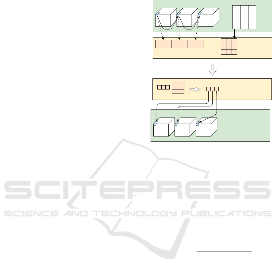
thread collaborations. When traversing along the n-

th dimension, the group of threads in a block stores

tensor ﬁber elements and m

dictionary elements

from the global memory to the shared memory, see

Figure 1. The inner product between a ﬁber and all

the columns in a dictionary is then computed on the

shared memory. The resulting ﬁber is stored at the

same location on the global memory due to the dicti-

onary being squared matrices.

Global memory

T(1,1,1,1) T(1,1,1,2) T(1,1,1,3)

Shared memory

(n)

Shared memoryU

(n)

T(1,1,1,:)

Global memory

X(1,1,1,:)

T(1,1,1,:)

Figure 1: The n-mode product on the GPU. Here T is a

4D-tensor and the ﬁrst thread is traversing along the fourth

dimension. Observe that this is just an illustration of the

concept, the data points are not explicitly stored as tensors

on the global memory.

3.2 Computing Sparse Coefﬁcient

Tensors

In this section we will cover how to transform the

norm of the n-mode product of a sparse tensor into

almost a single instruction, see line 10 in Algorithm

The Frobenius norm of a tensor X is the square

root of the sum of the squares of all its elements

∑

···

∑

...i

. (3)

Let the norm of a tensor be deﬁned as Equation 3.

Let

T = X ×

(1,k)

··· ×

(n,k)

X = T ×

(1,k)

)

··· ×

(n,k)

)

(4)

and

T = Y ×

(1,k)

··· ×

(n,k)

V = X − Y

< Y,V > = 0,

(5)

such that Y is a sparse version of X ,



(1,k)

...U

(n,k)



n=1

form orthonormal basis and

V is the complementary dense version of X with

respect to Y.

GPU Accelerated Sparse Representation of Light Fields

179

We will use the orthogonal invariance property

from



(1,k)

...U

(n,k)



n=1

, which preserves the norm, i.e

kX k

= < X ,X >

= < X ,T ×

(1,k)

)

··· ×

(n,k)

)

= < X ×

(1,k)

··· ×

(n,k)

,T >

= < T ,T >

= kT k

(6)

By using Equation 4 and Equation 5 we can now de-

ﬁne the problem as

kT −

T k

= kT k

− 2 < T ,

T > + k

T k

(7)

and for the inner product we have that

< T ,

T > = < T ,Y ×

(n,k)

··· ×

(1,k)

= < T ×

(1,k)

)

··· ×

(n,k)

)

,Y >

= < X , Y >

= < V + Y, Y >

= < V,Y > + < Y, Y >

= 0 + < Y, Y >

= kYk

(8)

With the property of orthogonality in Equation 6 and

Equation 8 we can rewrite Equation 7 to

kT −

T k

= kT k

− 2kYk

+ kYk

= kT k

− kYk

(9)

We can now take advantage of the result in Equa-

tion 9 in our iterative routine. Since Y is sparse and

we iteratively include one element at a time from X ,

we can break this down to an element-wise update.

We have from Equation 3, together with a linear in-

dex j of P as the total number of elements, that

kT k

∑

···

∑

...i

∑

j=1

(10)

By putting Equation 9 and Equation 10 together we

have

kT k

− kYk

∑

j=1

−

∑

l=1

(11)

We exploit the sparse structure of Y and iteratively

add one element at a time from X . Let 0 < M < τ,

where M is the number of nonzero coefﬁcients in the

sparse tensor Y at a speciﬁc iteration and τ is the spar-

sity paremeter. Then, from Equation 9 and the formu-

lation of Equation 11 together with the index l as the

location to the nonzero coefﬁcients, we ﬁnally have

kT k

− kYk

∑

j=1

−

∑

l=1

(12)

4 RESULTS

The results for the GPU implementation were

achieved with Nvidia GeForce GTX Titan Xp and

Intel Xeon CPU W3670 at 3.2 GHz. Since the

computations were performed on the GPU only one

CPU core was used.

The timings for the CPU version were obtained

by a machine with four Xeon E7-4870, a total of 40

cores at 2.4 GHz. The data sets we used to evalute

our method were acquired by Stanford University

(Computer Graphics Laboratory, 2018). For the

training of the dictionaries we used the following

light ﬁelds: Lego Truck, Chess, Eucalyptus Flowers,

Jelly Beans, Amethyst, Bunny, Treasure Chest and

Lego Bulldozer. In order to create 5D data points we

used the central 8x8 views of the light ﬁelds. The

data points of each data set have the dimensions m

5, m

= 5, m

= 3, m

= 8 and m

= 8.

For the testing set we used Lego Knights (1024x1024

image resolution), Tarot Cards and Crystal Ball

(1024x1024 image resolution) and Bracelet

(1024x680 image resolution), see Figure 2. We

used sparsity parameter τ = 300, τ = 390, τ = 412,

respectively for the three data sets. We set the

threshold parameter ε = 5 × 10

−5

, ε = 5 × 10

−5

and

ε = 7 × 10

−5

, respectively.

We show the encoding time of the presented met-

hod, see Table 1, where we compare CPU time and

GPU time. We evaluated our method with K = 64

number of dictionaries. The total encoding time for

the CPU for the three data sets are 124 seconds, 122

seconds and 83 seconds, respectively. Comparing this

to our GPU implementation we get 8.5 seconds, 8.3

seconds and 5.2 seconds. Normalizing these results

to K = 1, we get the following timings per dictionary:

133.2 ms for Lego Knights, 129.8 ms for Tarot Cards

and Crystal Ball and 81.6 ms for Bracelet. Compa-

red to the CPU timings: 1937 ms, 1906 ms and 1296

ms, respectively. As seen in Table 1, we get a sig-

niﬁcant computation speedup by processing the data

points segmentally in parallel on the GPU.

VISAPP 2019 - 14th International Conference on Computer Vision Theory and Applications

180

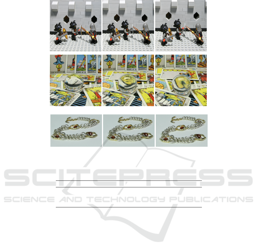
Figure 2: Reference views of the Lego Knights, Tarot Cards and Crystal Ball and Bracelet data sets.

Table 1: The measured time for the Lego Knights data set with K = 64 dictionaries, sparsity τ = 300 and threshold ε =

5 × 10

−5

. Further we have K = 64, τ = 390 and ε = 7 × 10

−5

for the Tarot Cards. Lastly, we have K = 64, τ = 412 and

ε = 5 × 10

−5

for the Bracelet data set.

Data set GPU Time (s) CPU Time (s) Speedup

Lego Knights 8.5 124 x14.54

Tarot Cards 8.3 122 x14.70

Bracelet 5.2 83 x15.90

5 CONCLUSIONS

We have presented a GPU accelerated light ﬁeld com-

pression method. The implemented method scales

in both memory and speed for higher dimensions -

which leads to faster computations, not only by faster

GPUs, but also by GPUs with larger memory. With

an order of magnitude faster computation speed, we

are able to produce a high quality compression that is

equivalent to the results of similar work in the rese-

arch ﬁeld.

We also show that computations on a single GPU

outperforms even massively parallel CPUs. For even

faster performance, multiple GPUs can be used simul-

taneously.

With very few changes we can use same imple-

mentation for the training phase on the GPU. This

would accelerate the creation of the dictionaries more.

REFERENCES

Adelson, E. H. and Bergen, J. R. (1991). The plenoptic

function and the elements of early vision. In Com-

putational Models of Visual Processing, pages 3–20.

MIT Press.

Aharon, M., Elad, M., and Bruckstein, A. (2006). k -svd:

An algorithm for designing overcomplete dictionaries

for sparse representation. Signal Processing, IEEE

Transactions on, 54(11):4311–4322.

Babacan, S., Ansorge, R., Luessi, M., Mataran, P. R., Mo-

lina, R., and Katsaggelos, A. K. (2012). Compressive

light ﬁeld sensing. IEEE Trans. on Image Processing,

21(12):4746–4757.

Choudhury, B., Swanson, R., Heide, F., Wetzstein, G., and

Heidrich, W. (2017). Consensus convolutional sparse

coding. In 2017 IEEE International Conference on

Computer Vision (ICCV), pages 4290–4298.

Computer Graphics Laboratory, S. U. (2018). Stanford uni-

versity - the (new) stanford light ﬁeld archive. http:

//lightﬁeld.stanford.edu/. Accessed: 2018-07-23.

Elad, M. (2010). Sparse and Redundant Representations:

GPU Accelerated Sparse Representation of Light Fields

181

From Theory to Applications in Signal and Image Pro-

cessing. Springer Publishing Company, Incorporated,

1st edition.

Jones, A., Nagano, K., Busch, J., Yu, X., Peng, H. Y., Bar-

reto, J., Alexander, O., Bolas, M., Debevec, P., and

Unger, J. (2016). Time-offset conversations on a life-

sized automultiscopic projector array. In 2016 IEEE

Conference on Computer Vision and Pattern Recogni-

tion Workshops (CVPRW), pages 927–935.

Kolda, T. G. and Bader, B. W. (2009). Tensor decompositi-

ons and applications. SIAM Review, 51(3):455–500.

Levoy, M. A. (2001). The digital michelangelo project.

Computer Graphics Forum, 18(3):xiii–xvi.

Liang, C.-K., Lin, T.-H., Wong, B.-Y., Liu, C., and Chen,

H. H. (2008). Programmable aperture photography:

multiplexed light ﬁeld acquisition. In Proc. of ACM

SIGGRAPH, volume 27, pages 1–10.

Miandji, E., Kronander, J., and Unger, J. (2013). Lear-

ning based compression of surface light ﬁelds for real-

time rendering of global illumination scenes. In SIG-

GRAPH Asia 2013 Technical Briefs, SA ’13, pages

24:1–24:4, New York, NY, USA. ACM.

Miandji, E., Kronander, J., and Unger, J. (2015). Compres-

sive image reconstruction in reduced union of subspa-

ces. Comput. Graph. Forum, 34(2):33–44.

Ng, R. (2005). Light ﬁeld photography with a hand-held

plenoptic camera. Computer Science Technical Report

CSTR 2, 11:1–11.

Vaish, V., Levoy, M., Szeliski, R., Zitnick, C. L., and Kang,

S. B. (2006). Reconstructing occluded surfaces using

synthetic apertures: Stereo, focus and robust measu-

res. In 2006 IEEE Computer Society Conference on

Computer Vision and Pattern Recognition (CVPR’06),

volume 2, pages 2331–2338.

Wanner, S. and Goldluecke, B. (2013). Variational light

ﬁeld analysis for disparity estimation and super-

resolution. IEEE Transactions of Pattern analysis and

machine intelligence, 36(3).

Wetzstein, G., Lanman, D., Hirsch, M., and Raskar, R.

(2012). Tensor displays: Compressive light ﬁeld synt-

hesis using multilayer displays with directional back-

lighting. ACM Trans. Graph., 31(4):80:1–80:11.

Williem, W. and Park, I. K. (2016). Robust light ﬁeld depth

estimation for noisy scene with occlusion. In 2016

IEEE Conference on Computer Vision and Pattern Re-

cognition (CVPR), pages 4396–4404.

VISAPP 2019 - 14th International Conference on Computer Vision Theory and Applications

182