Color Beaver: Bounding Illumination Estimations for Higher Accuracy

Karlo Ko

cevi

c, Nikola Bani

c and Sven Lon

cari

Image Processing Group, Department of Electronic Systems and Information Processing,

Faculty of Electrical Engineering and Computing, University of Zagreb, 10000 Zagreb, Croatia

Keywords:

Chromaticity, Color Constancy, Genetic Algorithm, Illumination Estimation, Image Enhancement, White

Balancing.

Abstract:

The image processing pipeline of most contemporary digital cameras performs illumination estimation in

order to remove the inﬂuence of illumination on image scene colors. In this paper an experiment is described

that examines some of the basic properties of illumination estimation methods for several Canon’s camera

models. Based on the obtained observations, an extension to any illumination estimation method is proposed

that under certain conditions alters the results of the underlying method. It is shown that with statistics-based

methods as underlying methods the proposed extension can outperform camera’s illumination estimation in

terms of accuracy. This effectively demonstrates that statistics-based methods can still be successfully used for

illumination estimation in digital cameras. The experimental results are presented and discussed. The source

code is available at https://ipg.fer.hr/ipg/resources/color

constancy.

1 INTRODUCTION

Among many abilities human visual system (HVS)

can recognize colors of objects regardless of scene

illumination. This ability is known as color con-

stancy (Ebner, 2007). Achieving computational co-

lor constancy is an important pre-processing step in

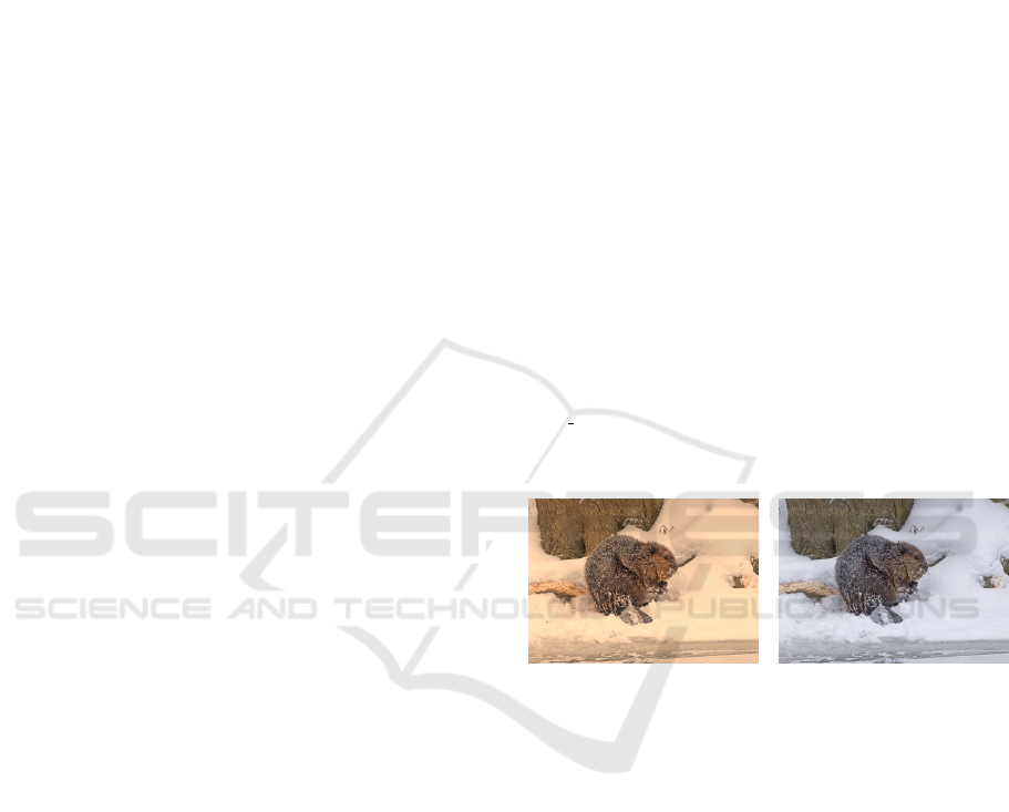
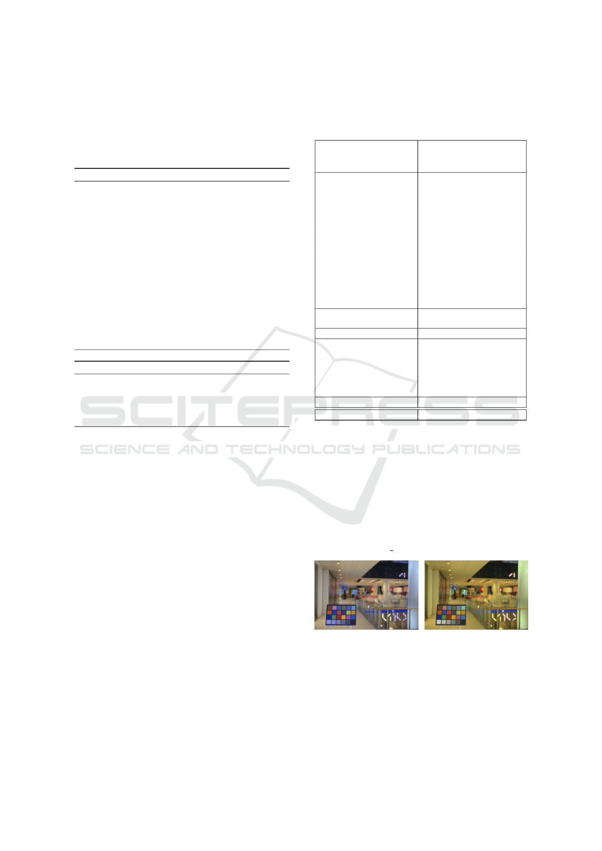
image processing pipeline as different scene illumina-

tions may cause the image colors to differ as shown in

ﬁgure 1. In order to remove the inﬂuence of illumina-

tion color, accurate illumination estimation followed

by chromatic adaptation must be preformed. For both

tasks the following image f formation model, which

includes Lambertian assumption, is most often used:

(x) =

I(λ, x)R(x, λ)ρ

(λ)dλ (1)

where c is a color channel, x is a given image

pixel, λ is the wavelength of the light, ω is the vi-

sible spectrum, I(λ, x) is the spectral distribution of

the light source, R(x, λ) is the surface reﬂectance, and

(λ) is the camera sensitivity of c-th color channel.

With the assumption of uniform illumination the pro-

blem can be simpliﬁed, as now x is removed from

I(λ, x) and the observed light source color is given

as:

e =









I(λ)ρ(λ)dλ (2)

(a) (b)

Figure 1: The same scene (a) with and (b) without illumi-

nation color cast.

For a successful chromatic adaptation, what is

required is only the direction of e (Barnard et al.,

2002). Since it is very common that only image pixel

values f are given and both I(λ) and ρ(λ) remain

unknown, calculating e is an ill-posed problem. To

solve this problem, additional assumptions must be

made, which leads to many color constancy methods

that are divided into two major groups. First group

of methods are low-level statistic-based methods like

White-patch (Land, 1977; Funt and Shi, 2010), its

improvements (Bani

c and Lon

cari

c, 2013; Bani

c and

Lon

cari

c, 2014a; Bani

c and Lon

cari

c, 2014b), Gray-

world (Buchsbaum, 1980), Shades-of-Gray (Finlay-

son and Trezzi, 2004), Gray-Edge (1st and 2nd or-

der) (Van De Weijer et al., 2007a), using bright and

dark colors (Cheng et al., 2014). The second group

is formed of learning-based methods like gamut map-

ping (pixel, edge, and intersection based) (Finlayson

Koš

cevi

c, K., Bani

c, N. and Lon

cari

c, S.

Color Beaver: Bounding Illumination Estimations for Higher Accuracy.

DOI: 10.5220/0007393701830190

In Proceedings of the 14th International Joint Conference on Computer Vision, Imaging and Computer Graphics Theory and Applications (VISIGRAPP 2019), pages 183-190

ISBN: 978-989-758-354-4

183

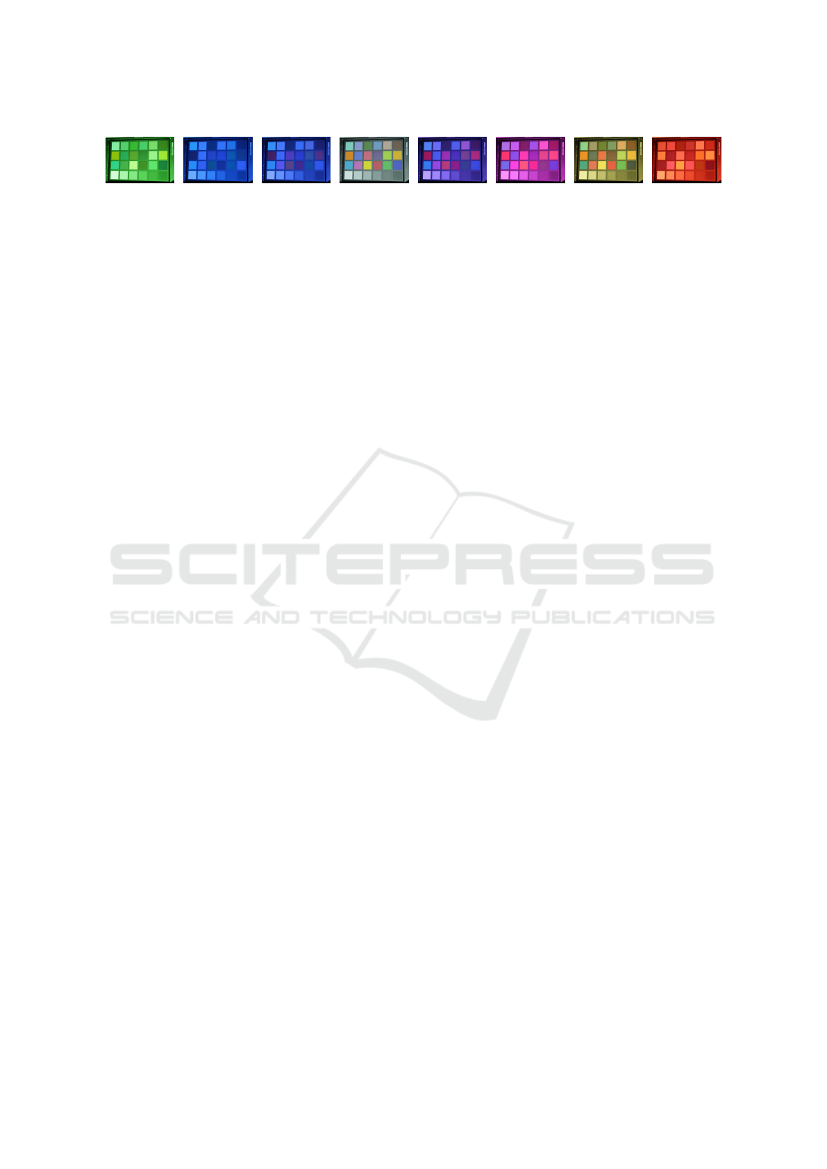
(a) (b) (c) (d) (e) (f) (g) (h)

Figure 2: Color checker cast with projector light of various colors.

et al., 2006), using high-level visual information (Van

De Weijer et al., 2007b), natural image statistics (Gi-

jsenij and Gevers, 2007), Bayesian learning (Gehler

et al., 2008), spatio-spectral learning (maximum li-

kelihood estimate, and with gen. prior) (Chakra-

barti et al., 2012), simplifying the illumination so-

lution space (Bani

c and Lon

cari

c, 2015a; Bani

c and

Lon

cari

c, 2015b; Bani

c and Lon

cari

c, 2015b), using

color/edge moments (Finlayson, 2013), using regres-

sion trees with simple features from color distribu-

tion statistics (Cheng et al., 2015), performing vari-

ous kinds of spatial localizations (Barron, 2015; Bar-

ron and Tsai, 2017), using convolutional neural net-

works (Bianco et al., 2015; Shi et al., 2016; Hu et al.,

2017; Qiu et al., 2018).

While learning-based method have a much higher

accuracy, it are low-level statistics-based methods that

are still being widely used among digital camera ma-

nufacturers since they are much faster and often more

hardware-friendly than learning-based methods. This

is also one of the reasons why statistics-based met-

hods are still important for research. Nevertheless,

since cameras are commercial systems, the fact that

they still widely use statistics-based methods is not

publicly stated. In this paper an experiment is des-

cribed that examines some of the basic properties of

illumination estimation methods for several Canon’s

camera models. Based on the obtained observations,

an extension to any illumination estimation method is

proposed that under certain conditions alters the re-

sults of the underlying method by bounding them to

a previously learned region in the chromaticity plane.

The bounding procedure is simple and does not add

any signiﬁcant cost to the overall computation. It is

shown that with statistics-based methods as under-

lying methods the proposed extension can outperform

camera’s built-in illumination estimation in terms of

accuracy. This effectively demonstrates that statistics-

based methods can still be successfully used for illu-

mination estimation in digital cameras’ pipelines.

The paper is structured as follows: Section 2 lays

out the motivation for the paper, in Section 3 the pro-

posed method is described, Section 4 shows the expe-

rimental results, and Section 5 concludes the paper.

2 MOTIVATION

2.1 Do statistics-based Methods

Matter?

Digital cameras are being used ever more widely, es-

pecially with the growing number of smartphones.

This deﬁnitely means that the results of the rese-

arch on computational color constancy now also have

a higher impact so the importance of this research

grows, especially when considering that it is an ill-

posed problem. In literature and in the reviews of

papers it is sometimes claimed that there is little pur-

pose in researching low-level statistics-based methods

since there are now much more accurate learning-

based methods that signiﬁcantly outperform them in

accuracy. In contrast to that many experts with ex-

perience in the industry claim that many commercial

white balancing systems are still based on low-level

statistics-based methods. The main reason for that

is their simplicity, low cost of implementation, and

hardware-friendliness. If this is indeed so, then the

research on such methods is deﬁnitely still important

and should be further conducted and supported.

To check to what degree all these claims are true, it

should be enough to examine some of the white balan-

cing systems widely used in commercial cameras. In

the world of professional cameras Canon has been the

market leader for 15 years (Canon, 2018) and in 2018

it held an estimated 49% of the market share (Pho-

toRumors, 2018). Since practically every digital ca-

mera performs white balancing in its image proces-

sing pipeline, it can be claimed that Canon’s white

balancing system is one of the most widely spread

ones. However, since Canon is a commercial com-

pany, full details of the white balancing system used

in its digital cameras are not publicly known.

2.2 Learning from Existing Systems

One approach to gain more information on Canon’s

white balancing system is to look at the results of il-

lumination estimation for various images taken under

illumination of numerous colors. The following three

camera models have been used to perform this expe-

riment: EOS 550D, EOS 6D, and EOS 750D.

VISAPP 2019 - 14th International Conference on Computer Vision Theory and Applications

184

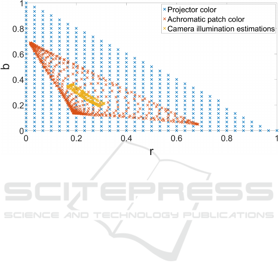
Figure 3: Comparison of chromaticities of projector light color, color of the second achromatic color checker patch, and

camera’s illumination estimation for Canon EOS 550D in the rb-chromaticity plane. The red chromaticity is shown on the x

axis, while the blue chromaticity is shown on the y axis.

The experiment was conducted in a dark room

where only a projector has been used as a light source.

The projector was used to cast illumination of vari-

ous colors, with chromaticities evenly spread in the

chromaticity plane, on a color checker as shown in Fi-

gure 2. These images of the color checker were taken

with every of the three previously mentioned cameras.

Although the illumination color was supposed to

be computationally determined by projecting speciﬁ-

cally created content, due to the projector and camera

sensor characteristics the effective illumination color

is altered. Its value as perceived by the camera can be

read from the achromatic patches in the last row of the

color checker and it serves as the ground-truth illumi-

nation for the given image. Ideally, it is this color that

an illumination estimation method should predict.

Finally, the last step of the experiment was to

check the results of illumination estimation perfor-

med by each of the cameras. The results of a ca-

mera’s illumination estimation for a taken image can

be reconstructed from the Exif metadata stored in the

image ﬁle. The ﬁelds needed for this are Red Balance

and Blue Balance, which have the values of channel

gains i.e. the factors by which the red and blue chan-

nels have to be multiplied to perform chromatic adap-

tation. For practical reasons in cameras the green gain

is ﬁxed to 1. The combined inverse values of these

gains give the illumination estimation vector. When

this vector is normalized, it represents the chromati-

city of camera’s illumination estimation, which can

be directly used to calculate the estimation accuracy

by comparing it to the ground-truth illumination.

A comparison between the chromaticities for pro-

jected illumination color, achromatic patch color,

and camera illumination estimations for Canon EOS

550D camera is given in Figure 3. The values read

from achromatic white patches are squeezed with re-

spect to the ones sent by the projector, but a more in-

teresting observation is that none of the camera’s il-

lumination estimation are outside of a surface that re-

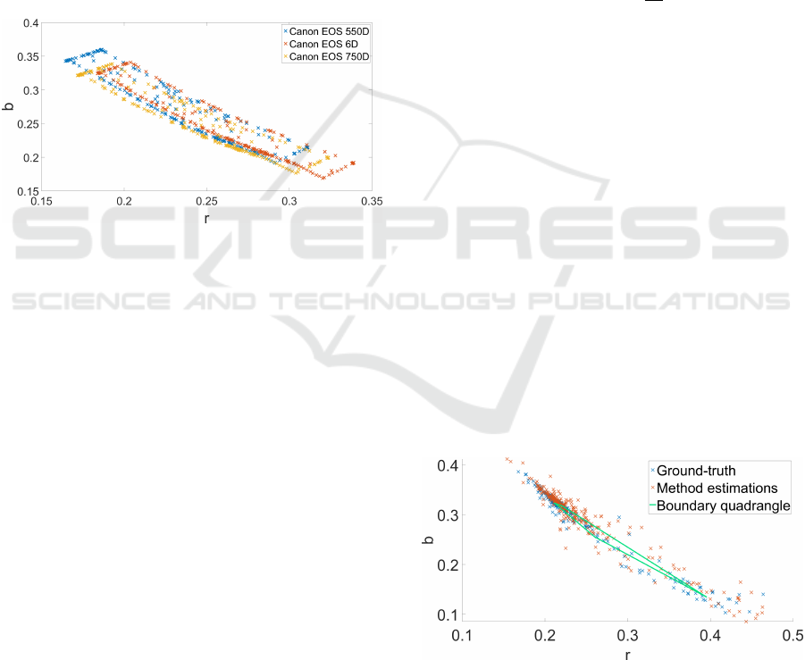
sembles a parallelogram. As shown in Figure 4, simi-

lar results are obtained for other used camera models

as well. Although there are some differences between

the parallelograms mostly visible on two opposite si-

des, the parallelograms otherwise mostly cover a si-

milar space in the chromaticity plane.

2.3 Observations

Based on these observations it can be concluded that

one of the core properties of Canon’s white balancing

system is limiting its illumination estimation so that

they do not appear outside of a polygon very similar

to a parallelogram. Such limitation can be justiﬁed by

the goal of avoiding unlikely illuminations and thus

minimizing the occurrence of too high errors. This

can be useful if it can be assumed that the expected

illuminations are similar to black body radiation, but

Color Beaver: Bounding Illumination Estimations for Higher Accuracy

185

sometimes it can be an disadvantage if artiﬁcially co-

lored illumination sources are present like in Figure 2.

On the other hand, there is little that can be said

about the white balancing system’s behavior inside of

the parallelogram. Nevertheless, the limitation obser-

vation is already useful because of its potential to li-

mit maximum errors for illumination estimations. As

for the behavior of illumination estimation inside the

parallelogram, a possible solution is to use some of

the already existing methods. Additionally, it can be

immediately remarked that a parallelogram is a rela-

tively regular quadrangle and polygon in general.

At least two questions can be raised here: ﬁrst, is

there a better quadrangle i.e. polygon for bounding

the illuminations, and second, which method to use

as the baseline underlying method that gets bounded?

Figure 4: Comparison of cameras’ illumination estimation

for Canon EOS 550D, Canon EOS 6D, and Canon EOS

750D. The red chromaticity is shown on the x axis, while

the blue chromaticity is shown on the y axis.

3 PROPOSED METHOD

Inspired by the bounds used by Canon cameras ob-

served in Figure 4 and in order to give an answer to

the two questions from the previous section, in this

paper a new method i.e. extension to any chosen un-

derlying illumination estimation method is proposed.

The extension learns a bounding polygon with an ar-

bitrary number of vertices that is used to restrict the

illumination estimations of the initially chosen under-

lying method to the chromaticity region speciﬁed by

the bounding polygon. As explained in the previous

section, the motivation for this are the observations

of boundaries used by Canon cameras and it can be

applied to any illumination estimation method.

A genetic algorithm is used to learn the bounda-

ries. First, the illumination estimations for the ini-

tially chosen underlying method are calculated on a

given set of images. The boundary polygon popula-

tion of size s is initialized by taking randomly chosen

ground-truth illumination chromaticities as polygon

vertices. Empirically, it has been shown that the four-

point polygons i.e. quadrangles are generally a good

ﬁt for illumination restriction and there is no signiﬁ-

cant gain when the number of points is increased. The

ﬁtness function calculation for a given quadrangle is

based on the ground-truth illuminations and the re-

stricted illuminations that are the result of applying

the boundary polygon to the underlying method’s il-

lumination estimations. Empirically, it has been con-

cluded that the negative sum of the median angular

error and a tenth of the maximum angular error is ge-

nerally a good ﬁtness function; angular error is ex-

plained in more detail in Section 4.1. More formally,

if A = {a

, . . . , a

} is the set of angular errors on n

images, then the chosen ﬁtness function is given as

f(A) = −



med(A) +

max(A)



. (3)

The maximum error was also included in the ﬁt-

ness function in order to discourage quadrangles that

perform very well on the majority of the images, but

have poor performance of several outliers. As the se-

lection method the 3-way tournament selection (Mit-

chell, 1998) with random sampling is used. Avera-

ging crossover function of the two of the best indi-

viduals produces a new child which is randomly mu-

tated. The quadrangle with the lowest ﬁtness value

among the three ones chosen in the selection proce-

dure is replaced in the current population by the ne-

wly created child quadrangle. The mutation is done

by translating each vertex of a bounding polygon by

the value from the normal distribution with µ = 0

and σ = 0.2. Mutation rate, which states whether the

whole individual should me mutated, is set to 0.3. Af-

ter all training iterations have ﬁnished, the boundary

quadrangle with the highest ﬁtness value is chosen as

the ﬁnal result. Figure 5 shows an example of a lear-

ned quadrangle.

Figure 5: Example of a learned boundary quadrangle for

the Canon1 dataset (Cheng et al., 2014) in the chromaticity

plane. The red chromaticity is shown on the x axis, while

the blue chromaticity is shown on the y axis.

Since the proposed extension bounds illumination

estimations and beavers are known to bound water

VISAPP 2019 - 14th International Conference on Computer Vision Theory and Applications

186

ﬂows by building dams, the proposed extension was

named Color Beaver. In the rest of the paper exten-

ding a method M by the Color Beaver extension will

be denoted as Color Beaver + M. The training proce-

dure for Color Beaver is summarized in Algorithm 2.

Algorithm 1: Color Beaver Training.

Input: training images I, ground truth G, met-

hod M, iterations number N, population size s, ﬁtness

function f

Output: boundary polygon P

1: E = estimateIllumination(I, M)

2: P = initializePolygonPopulation(s)

3: for i ∈ {1, ..N} do

4: t

, t

= tournamentSelection(P, 3, f)

5: t

= crossover(t

, t

)

6: t

.mutateMaybe(0.3)d

7: R = restrictIllumination(E, t

)

8: P.ReplaceExistingWith(t

, t

)

9: end for

10: P = P.GetFittest(f)

Algorithm 2: Color Beaver Application.

Input: image I, method M, boundary polygon P

Output: illumination estimation e

1: e

= estimateIllumination(I, M)

2: e = restrictIllumination(e

, P)

4 EXPERIMENTAL RESULTS

4.1 Experimental Setup

Eight linear NUS datasets (Cheng et al., 2014) and the

Cube dataset (Bani

c and Lon

cari

c, 2017) have been

used to test the proposed extension and compare its

performance to the one of other methods. All these

datasets have linear images, which is also expected

by the model described by Eq. (3). The ColorChecker

dataset (Gehler et al., 2008; Shi and Funt, 2018) has

not been used because of much confusion that is still

present in many papers due to of its misuses in the

past (Lynch et al., 2013; Finlayson et al., 2017).

The most commonly used accuracy measure

among many proposed (Gijsenij et al., 2009; Finlay-

son and Zakizadeh, 2014; Bani

c and Lon

cari

c, 2015a)

is the angular error. It is the angle between the vectors

of illumination estimation and the ground-truth illu-

mination. When the angular errors obtained on each

individual image of a given benchmark dataset need

to be summarized, one of the most important statistics

is the median angular error (Hordley and Finlayson,

Table 1: Performance of different color constancy methods

on the Cube dataset (Bani

c and Lon

cari

c, 2017) in terms

of angular error statistics (lower Avg. is better). The used

format is the same as in (Barron and Tsai, 2017).

Algorithm MeanMed. Tri.

Best

25%

Worst

25%

Avg.

White-Patch (Funt and Shi,

2010)

6.58 4.48 5.27 1.18 15.23 4.88

Gray-world (Buchsbaum, 1980) 3.75 2.91 3.15 0.69 8.18 2.87

Camera built-in 2.96 2.56 2.64 0.82 5.79 2.49

Color Tiger (Bani

c and Lon

cari

2017)

2.94 2.59 2.66 0.61 5.88 2.35

Shades-of-Gray (Finlayson and

Trezzi, 2004)

2.58 1.79 1.95 0.38 6.19 1.84

2nd-order Gray-Edge (Van

De Weijer et al., 2007a)

2.49 1.60 1.80 0.49 6.00 1.84

1st-order Gray-Edge (Van

De Weijer et al., 2007a)

2.45 1.58 1.81 0.48 5.89 1.81

General Gray-World (Barnard

et al., 2002)

2.50 1.61 1.79 0.37 6.23 1.76

Color Beaver Camera +

built-in (proposed)

1.70 0.96 1.15 0.31 4.38 1.20

Color Beaver + WP (proposed) 1.59 0.87 1.04 0.25 4.15 1.08

Restricted Color Tiger (Bani

and Lon

cari

c, 2017)

1.64 0.82 1.05 0.24 4.37 1.08

Color Dog (Bani

c and Lon

cari

2015b)

1.50 0.81 0.99 0.27 3.86 1.05

Smart Color Cat (Bani

c and

Lon

cari

c, 2015b)

1.49 0.88 1.06 0.24 3.75 1.04

Color Beaver + SoG (proposed) 1.51 0.81 1.00 0.22 3.97 1.01

Color Beaver + GW (proposed) 1.48 0.76 0.98 0.21 3.90 0.98

2004). Despite that fact, the geometric mean of se-

veral statistics including the median angular error has

increasingly been gaining popularity in recent publi-

cations (Barron and Tsai, 2017) and the same format

as there is also used in this paper.

For both the NUS datasets and the Cube data-

set a three-fold cross-validation with folds of equal

size was used like in previous publications. The

source code for recreating the results reported later

in the paper is publicly available at https://ipg.fer.hr/

ipg/resources/color constancy.

(a) (b)

Figure 6: A failure case for Color Beaver + SoG with chro-

matic adaptation results based on a) the restricted illumi-

nation estimation with angular error of 10.74

◦

and b) the

ground-truth illumination.

Color Beaver: Bounding Illumination Estimations for Higher Accuracy

187

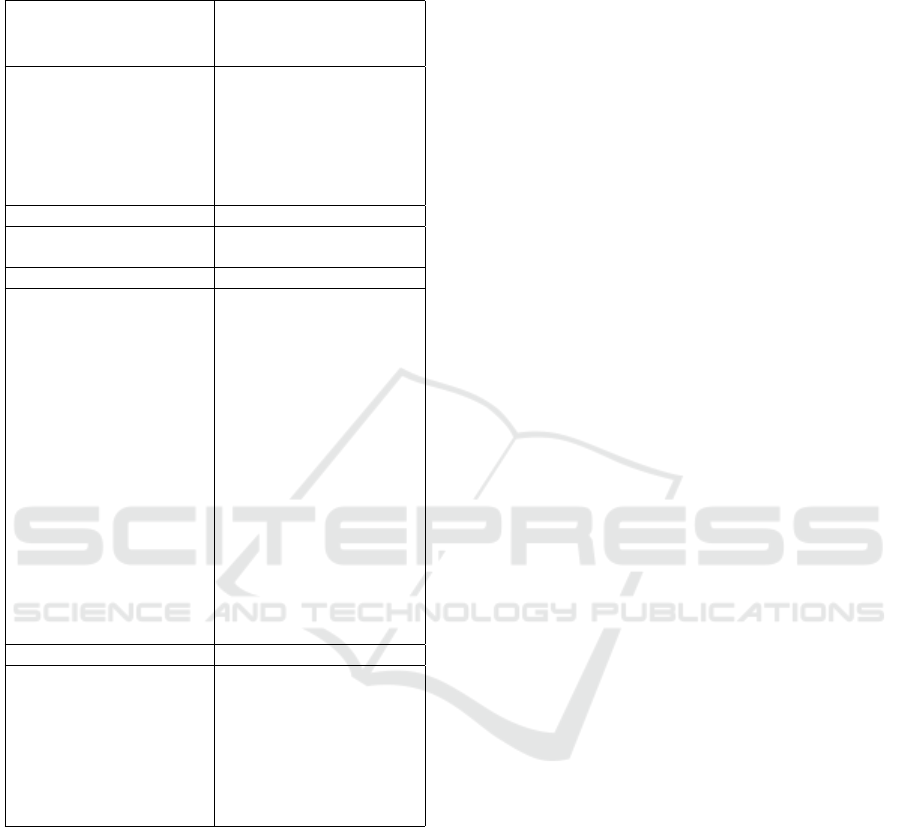
Table 2: Combined performance of different color con-

stancy methods on eight NUS dataset in terms of angular

error statisrics (lower Avg. is better). The used format is

the same as in (Barron and Tsai, 2017).

Algorithm MeanMed. Tri.

Best

25%

Worst

25%

Avg.

White-Patch (Funt and Shi,

2010)

9.91 7.44 8.78 1.44 21.27 7.24

Pixels-based Gamut (Gijsenij

et al., 2010)

5.27 4.26 4.45 1.28 11.16 4.27

Grey-world (Buchsbaum, 1980) 4.59 3.46 3.81 1.16 9.85 3.70

Edge-based Gamut (Gijsenij

et al., 2010)

4.40 3.30 3.45 0.99 9.83 3.45

Color Beaver + WP (proposed) 5.40 2.12 2.75 0.58 16.08 3.12

Shades-of-Gray (Finlayson and

Trezzi, 2004)

3.67 2.94 3.03 0.98 7.75 3.01

Color Beaver + GW (proposed) 3.73 2.65 2.90 0.72 8.55 2.82

Natural Image Statistics (Gijsenij

and Gevers, 2011)

3.45 2.88 2.95 0.83 7.18 2.81

Local Surface Reﬂectance

Statistics (Gao et al., 2014)

3.45 2.51 2.70 0.98 7.32 2.79

2nd-order Gray-Edge (Van

De Weijer et al., 2007a)

3.36 2.70 2.80 0.89 7.14 2.76

1st-order Gray-Edge (Van

De Weijer et al., 2007a)

3.35 2.58 2.76 0.79 7.18 2.67

Bayesian (Gehler et al., 2008) 3.50 2.36 2.57 0.78 8.02 2.66

General Gray-World (Barnard

et al., 2002)

3.20 2.56 2.68 0.85 6.68 2.63

Spatio-spectral

Statistics (Chakrabarti et al.,

2012)

3.06 2.58 2.74 0.87 6.17 2.59

Bright-and-dark Colors

PCA (Cheng et al., 2014)

2.93 2.33 2.42 0.78 6.13 2.40

Corrected-Moment (Finlayson,

2013)

2.95 2.05 2.16 0.59 6.89 2.21

Color Beaver + SoG (proposed) 2.86 1.99 2.21 0.59 6.62 2.17

Color Tiger (Bani

c and Lon

cari

2017)

2.96 1.70 1.97 0.53 7.50 2.09

Color Dog (Bani

c and Lon

cari

2015b)

2.83 1.77 2.03 0.48 7.04 2.03

Shi et al. 2016 (Shi et al., 2016) 2.24 1.46 1.68 0.48 6.08 1.74

CCC (Barron, 2015) 2.38 1.48 1.69 0.45 5.85 1.74

Cheng 2015 (Cheng et al., 2015) 2.18 1.48 1.64 0.46 5.03 1.65

FFCC (Barron and Tsai, 2017) 1.99 1.31 1.43 0.35 4.75 1.44

4.2 Accuracy

Tables 1 and 2 show the comparisons between the

accuracies of methods extended by the proposed ex-

tension and other illumination estimation methods. It

can be seen that all of the extended methods outper-

form their initial non-extended versions. As a mat-

ter of fact, the extended version of the Shades-of-

Gray method outperforms the camera built-in method.

Additionally, the extended versions also outperform

many learning-based methods. All these results de-

monstrate the usability of the proposed extension. An

example of a failure case for the proposed extension

of Shades-of-Gray is shown in Figure 6.

While other methods such as Gray-edge could

also have been tested and shown in the Tables,

Shades-of-Gray was already good enough to outper-

form camera’s built-in methods. Extending Gray-

edge also increases its accuracy, but Gray-edge is slo-

wer than Shades-of-Gray (Cheng et al., 2014), more

complex, and it requires additional memory. Hence

it was left out of the testing procedures since Shades-

of-Gray is already sufﬁcient to successfully answer

the questions that were raised in this paper.

4.3 Discussion

The fact that statistics-based methods extended by the

proposed method outperform camera built-in illumi-

nation estimation methods is signiﬁcant for drawing

further conclusions about the nature of camera’s il-

lumination estimation methods. Namely, if extended

statistics-based methods outperform them, it can be

freely stated that statistics-based are good enough to

be used in digital cameras. Additionally, it may be

that the extended method managed to outperform the

camera’s built-in methods because that they are also

statistics-based, which in turn conﬁrms that cameras

do indeed use such method. In any of these two cases

it can be concluded that research on statistics-based

methods still has a large ﬁeld of applications and the

obtained results only further prove its importance.

5 CONCLUSIONS

An experiment was conducted to examine some of the

details of built-in illumination estimation methods for

several Canon camera models. Inspired by the ob-

served results, an extension to any underlying illumi-

nation estimation method has been proposed. It li-

mits the values of the illumination estimations of the

underlying method by forcing it to stay inside a pre-

viously learned region in the chromaticity plane wit-

hout adding any signiﬁcant computation cost. By li-

miting some of the best-known statistics-based met-

hods, the obtained accuracy outperforms the one of

cameras’ built-in methods. This effectively demon-

strates that by only using slightly modiﬁed statistics-

based methods it is possible to be more accurate than

contemporary cameras. It also proves the claim that

statistics-based methods can and probably are used

for illumination estimation in digital cameras. Future

research will include looking for new method modiﬁ-

cations that result in even higher estimation accuracy.

VISAPP 2019 - 14th International Conference on Computer Vision Theory and Applications

188

ACKNOWLEDGEMENTS

This work has been supported by the Croatian Science

Foundation under Project IP-06-2016-2092.

REFERENCES

Bani

c, N. and Lon

cari

c, S. (2015a). Color Cat: Remembe-

ring Colors for Illumination Estimation. Signal Pro-

cessing Letters, IEEE, 22(6):651–655.

Bani

c, N. and Lon

cari

c, S. (2015b). Using the red chroma-

ticity for illumination estimation. In Image and Signal

Processing and Analysis (ISPA), 2015 9th Internatio-

nal Symposium on, pages 131–136. IEEE.

Bani

c, N. and Lon

cari

c, S. (2017). Unsupervised

Learning for Color Constancy. arXiv preprint

arXiv:1712.00436.

Bani

c, N. and Lon

cari

c, S. (2013). Using the Random

Sprays Retinex Algorithm for Global Illumination Es-

timation. In Proceedings of The Second Croatian

Computer Vision Workshopn (CCVW 2013), pages 3–

7. University of Zagreb Faculty of Electrical Engi-

neering and Computing.

Bani

c, N. and Lon

cari

c, S. (2014a). Color Rabbit: Gui-

ding the Distance of Local Maximums in Illumina-

tion Estimation. In Digital Signal Processing (DSP),

2014 19th International Conference on, pages 345–

350. IEEE.

Bani

c, N. and Lon

cari

c, S. (2014b). Improving the White

patch method by subsampling. In Image Processing

(ICIP), 2014 21st IEEE International Conference on,

pages 605–609. IEEE.

Bani

c, N. and Lon

cari

c, S. (2015a). A Perceptual Measure

of Illumination Estimation Error. In VISAPP, pages

136–143.

Bani

c, N. and Lon

cari

c, S. (2015b). Color Dog: Guiding the

Global Illumination Estimation to Better Accuracy. In

VISAPP, pages 129–135.

Barnard, K., Cardei, V., and Funt, B. (2002). A compa-

rison of computational color constancy algorithms. i:

Methodology and experiments with synthesized data.

Image Processing, IEEE Transactions on, 11(9):972–

984.

Barron, J. T. (2015). Convolutional Color Constancy. In

Proceedings of the IEEE International Conference on

Computer Vision, pages 379–387.

Barron, J. T. and Tsai, Y.-T. (2017). Fast Fourier Color

Constancy. In Computer Vision and Pattern Recogni-

tion, 2017. CVPR 2017. IEEE Computer Society Con-

ference on, volume 1. IEEE.

Bianco, S., Cusano, C., and Schettini, R. (2015). Color

Constancy Using CNNs. In Proceedings of the IEEE

Conference on Computer Vision and Pattern Recogni-

tion Workshops, pages 81–89.

Buchsbaum, G. (1980). A spatial processor model for object

colour perception. Journal of The Franklin Institute,

310(1):1–26.

Canon (2018). Canon celebrates 15th consecutive year of

No.1 share of global interchangeable-lens digital ca-

mera market.

Chakrabarti, A., Hirakawa, K., and Zickler, T. (2012). Color

constancy with spatio-spectral statistics. Pattern Ana-

lysis and Machine Intelligence, IEEE Transactions on,

34(8):1509–1519.

Cheng, D., Prasad, D. K., and Brown, M. S. (2014). Illu-

minant estimation for color constancy: why spatial-

domain methods work and the role of the color distri-

bution. JOSA A, 31(5):1049–1058.

Cheng, D., Price, B., Cohen, S., and Brown, M. S. (2015).

Effective learning-based illuminant estimation using

simple features. In Proceedings of the IEEE Confe-

rence on Computer Vision and Pattern Recognition,

pages 1000–1008.

Ebner, M. (2007). Color Constancy. The Wiley-IS&T Se-

ries in Imaging Science and Technology. Wiley.

Finlayson, G. D. (2013). Corrected-moment illuminant es-

timation. In Proceedings of the IEEE International

Conference on Computer Vision, pages 1904–1911.

Finlayson, G. D., Hemrit, G., Gijsenij, A., and Gehler, P.

(2017). A Curious Problem with Using the Colour

Checker Dataset for Illuminant Estimation. In Color

and Imaging Conference, volume 2017, pages 64–69.

Society for Imaging Science and Technology.

Finlayson, G. D., Hordley, S. D., and Tastl, I. (2006). Ga-

mut constrained illuminant estimation. International

Journal of Computer Vision, 67(1):93–109.

Finlayson, G. D. and Trezzi, E. (2004). Shades of gray

and colour constancy. In Color and Imaging Confe-

rence, volume 2004, pages 37–41. Society for Ima-

ging Science and Technology.

Finlayson, G. D. and Zakizadeh, R. (2014). Reproduction

angular error: An improved performance metric for

illuminant estimation. perception, 310(1):1–26.

Funt, B. and Shi, L. (2010). The rehabilitation of MaxRGB.

In Color and Imaging Conference, volume 2010,

pages 256–259. Society for Imaging Science and

Technology.

Gao, S., Han, W., Yang, K., Li, C., and Li, Y. (2014). Ef-

ﬁcient color constancy with local surface reﬂectance

statistics. In European Conference on Computer Vi-

sion, pages 158–173. Springer.

Gehler, P. V., Rother, C., Blake, A., Minka, T., and Sharp, T.

(2008). Bayesian color constancy revisited. In Com-

puter Vision and Pattern Recognition, 2008. CVPR

2008. IEEE Conference on, pages 1–8. IEEE.

Gijsenij, A. and Gevers, T. (2007). Color Constancy using

Natural Image Statistics. In CVPR, pages 1–8.

Gijsenij, A. and Gevers, T. (2011). Color constancy using

natural image statistics and scene semantics. IEEE

Transactions on Pattern Analysis and Machine Intel-

ligence, 33(4):687–698.

Gijsenij, A., Gevers, T., and Lucassen, M. P. (2009). Per-

ceptual analysis of distance measures for color con-

stancy algorithms. JOSA A, 26(10):2243–2256.

Gijsenij, A., Gevers, T., and Van De Weijer, J. (2010).

Generalized gamut mapping using image derivative

Color Beaver: Bounding Illumination Estimations for Higher Accuracy

189

structures for color constancy. International Journal

of Computer Vision, 86(2):127–139.

Hordley, S. D. and Finlayson, G. D. (2004). Re-evaluating

colour constancy algorithms. In Pattern Recognition,

2004. ICPR 2004. Proceedings of the 17th Internatio-

nal Conference on, volume 1, pages 76–79. IEEE.

Hu, Y., Wang, B., and Lin, S. (2017). Fully Convolutional

Color Constancy with Conﬁdence-weighted Pooling.

In Computer Vision and Pattern Recognition, 2017.

CVPR 2017. IEEE Conference on, pages 4085–4094.

IEEE.

Land, E. H. (1977). The retinex theory of color vision.

Scientiﬁc America.

Lynch, S. E., Drew, M. S., and Finlayson, k. G. D. (2013).

Colour Constancy from Both Sides of the Shadow

Edge. In Color and Photometry in Computer Vision

Workshop at the International Conference on Compu-

ter Vision. IEEE.

Mitchell, M. (1998). An introduction to genetic algorithms.

MIT press.

PhotoRumors (2018). 2018 Canon, Nikon and Sony market

share (latest Nikkei, BCN and CIPA reports).

Qiu, J., Xu, H., Ma, Y., and Ye, Z. (2018). PILOT:

A Pixel Intensity Driven Illuminant Color Estima-

tion Framework for Color Constancy. arXiv preprint

arXiv:1806.09248.

Shi, L. and Funt, B. (2018). Re-processed Version of the

Gehler Color Constancy Dataset of 568 Images.

Shi, W., Loy, C. C., and Tang, X. (2016). Deep Specialized

Network for Illuminant Estimation. In European Con-

ference on Computer Vision, pages 371–387. Springer.

Van De Weijer, J., Gevers, T., and Gijsenij, A. (2007a).

Edge-based color constancy. Image Processing, IEEE

Transactions on, 16(9):2207–2214.

Van De Weijer, J., Schmid, C., and Verbeek, J. (2007b).

Using high-level visual information for color con-

stancy. In Computer Vision, 2007. ICCV 2007. IEEE

11th International Conference on, pages 1–8. IEEE.

VISAPP 2019 - 14th International Conference on Computer Vision Theory and Applications

190