Real-time 3D Pose Estimation from Single Depth Images
Thomas Schn
¨
urer
1,2
, Stefan Fuchs
2
, Markus Eisenbach
1
and Horst-Michael Groß
1
1
Neuroinformatics and Cognitive Robotics Lab, Ilmenau University of Technology, 98684 Ilmenau, Germany
2
Honda Research Institute Europe GmbH, 63073 Offenbach/Main, Germany
Keywords:
Real-time 3D Joint Estimation, Human-Robot-Interaction, Deep Learning.
Abstract:
To allow for safe Human-Robot-Interaction in industrial scenarios like manufacturing plants, it is essential
to always be aware of the location and pose of humans in the shared workspace. We introduce a real-time
3D pose estimation system using single depth images that is aimed to run on limited hardware, such as a
mobile robot. For this, we optimized a CNN-based 2D pose estimation architecture to achieve high frame
rates while simultaneously requiring fewer resources. Building upon this architecture, we extended the system
for 3D estimation to directly predict Cartesian body joint coordinates. We evaluated our system on a newly
created dataset by applying it to a specific industrial workbench scenario. The results show that our system’s
performance is competitive to the state of the art at more than five times the speed for single person pose
estimation.
1 INTRODUCTION
For scenarios in which intelligent systems are me-
ant to interact with humans, knowledge about the hu-
man’s state is vital. For example, location and posture
are important cues to reason about the activity and in-
tentions of a human. Especially in the case of human-
robot-collaboration and shared workspaces accurate
knowledge about the human’s 3D position is very im-
portant for both action planning and safety require-
ments.
Such a scenario may also introduce a number of
other constraints. For example, a lot of occlusions
might be caused by the workplace or construction
parts. Many state of the art approaches, however, are
sensitive to large amounts of occlusions. Even though
2D pose estimation attracted a lot of research interest
in the last decade, fewer attempt 3D pose estimation.
Also, many pose estimation systems only recently re-
ached real-time performance and usually still need a
considerable amount of resources (e.g. , OpenPose
(Cao et al., 2017) requires four Nvidia GTX 1080 de-
vices to run at ≈30 fps)
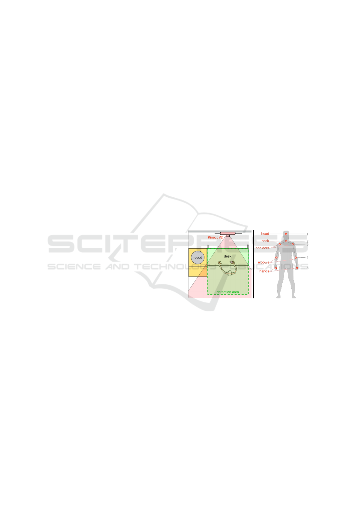
We have developed our approach by taking into
account requirements of an industrial workbench sce-
nario for human-robot-cooperation as shown in Fig. 1
(left). Here, a robot assists a human worker perfor-
ming tasks at a shared workbench while a depth ca-
mera is used to constantly monitor the human’s pose.
Figure 1: Left: Our industrial workbench scenario for
Human-Robot-Interaction. A keyboard, several movable
objects and a set of big buttons are placed on the desk as
means for interaction. Right: The eight upper body joints
(red) to be estimated by our system and their location in the
kinematic chain (grey).
For simplification, this camera is fixed above the desk,
but can also be installed on a mobile robot later on.
Since the lower part of the body is occluded by the
work bench, the pose estimation must work reliably
using only the eight upper body joints as shown in
Fig. 1 (right). Additionally, the hands and other body
parts might be occluded while handling objects. Our
approach addresses these points with corresponding
training data and output dimensions. Nevertheless, it
can be extended to other scenarios with an increased
number of joints.
Targeting the described scenario, we introduce
a real-time 3D pose estimation system using single
716
Schnürer, T., Fuchs, S., Eisenbach, M. and Groß, H.
Real-time 3D Pose Estimation from Single Depth Images.
DOI: 10.5220/0007394707160724
In Proceedings of the 14th International Joint Conference on Computer Vision, Imaging and Computer Graphics Theory and Applications (VISIGRAPP 2019), pages 716-724
ISBN: 978-989-758-354-4
Copyright
c
2019 by SCITEPRESS – Science and Technology Publications, Lda. All rights reserved

depth images on a mobile platform. Our approach is
based on a state of the art architecture for 2D pose
estimation which we improve regarding two main as-
pects: First, we propose optimization steps for sub-
stantial size reduction and speed improvements. Se-
cond, we extend the architecture for 3D pose estima-
tion. After training the resulting system on a newly
created dataset we compare different alternatives and
finally deploy the system in our scenario.
2 RELATED WORK
The majority of approaches focuses on 2D human
pose estimation in single RGB images. However,
for human-robot-interaction a 3D estimation is neces-
sary. Naturally, 2D images lack distance information,
which makes 3D pose estimation a much more diffi-
cult task. Approaches like (Elhayek et al., 2015) show
that multiple cameras can be used to overcome the li-
mitations of 2D images. This, however, requires a
more complicated camera setup, which is not accep-
table in many applications, e.g. , on a mobile robot.
Even though there are single camera approaches
that try to estimate the 3D position of joints based on
single 2D RGB images (Tekin et al., 2017) (Li and
Chan, 2015), they rely on additional information like
bone lengths (Mehta et al., 2017) or lack in precision
(Martinez et al., 2017). Only a few approaches try
to exploit depth information for 3D pose estimation.
They rely on additional knowledge, like a database
of possible poses (Baak et al., 2011), a volumetric hu-
man model (Zhang et al., 2012) or a good background
segmentation (Shotton et al., 2013).
However, the performance of such systems is al-
ways limited by the quality of their model and its
ability to generalize without additional information.
With the great success of deep Convolutional Neu-
ral Networks (deep CNNs) in this field, many recent
approaches successfully solve the task in 2D with
a model-free discriminative architecture (Toshev and
Szegedy, 2013) (Tekin et al., 2017) (Chu et al., 2017)
(Rafi et al., 2016). Most recently, some approaches
try to use a human model implicitly by adding auxi-
liary tasks like bone length estimation (Mehta et al.,
2017) or body part affinity (Cao et al., 2017). Here,
we compare a model-free method to one using an im-
plicit model in Sec. 4.
Regarding the estimation result, two main strate-
gies can be found. In 2D human pose estimation, it
is common practice to formulate the problem as a de-
tection task, where belief maps decode the probability
for each pixel to contain a certain joint. In 3D human
pose estimation, however, several approaches (Mar-
Figure 2: We used the basic Hourglass Block of (Newell
et al., 2016), but reduced the weights by 55% while main-
taining performance.
tinez et al., 2017) (Bulat and Tzimiropoulos, 2016)
solve it as a regression problem by finding the 3D
coordinates (x, y, z) as exact as possible.
In this paper, we use a state of the art model-free
deep CNN architecture for 2D joint detection in single
depth images, optimize it in regards to size and speed
and extend it to 3D estimation. Finally, we deploy
our system to the Robot Operating System (ROS) and
compare it to a method that uses an implicit model for
regression.
3 METHOD
We propose a lightweight system for real-time 3D
pose estimation shown in Fig. 3. It consists of two
stages for successive 2D and 3D estimation.
First, a Slim Stacked Hourglass CNN (SSHG 2D,
see Sec. 3.2) produces one 2D belief map H
j
∈ R
64x64
for each joint j ∈ {1... J} from a single depth image.
By calculating the weighted center of belief map acti-
vation, each joint’s 2D location p
2D
j
= {x
j
,y
j
} is esti-
mated.
Second, a refined depth map D
j
∈ R
64x64
is esti-
mated for each joint j, denoting its distance to the ca-
mera. In contrast to the input depth image, these refi-
ned depth maps allow for a higher precision, as descri-
bed in Sec. 3.3. The 3D pose p
3D
j
is then reconstructed
by retrieving the joint distance d
j
from its depth map
D
j
at its 2D location p
2D
j
, so that d
j
= D
j,x
j
,y
j
. Finally,
the joint location in camera coordinates {x
j
,y
j
,d
j
} is
projected into world coordinates p
3D
j
= {x
w
j
,y
w
j
,z
w
j
}
using the projection M(x
j
,y
j
,d
j
,CM) with CM being
the camera matrix.
3.1 Stacked Hourglass for 2D
Estimation
The Stacked Hourglass architecture introduced in
(Newell et al., 2016) uses multiple successive Hour-
glass Blocks like the one shown in Fig. 2 to produce
belief maps from single images. Being used in five of
Real-time 3D Pose Estimation from Single Depth Images
717
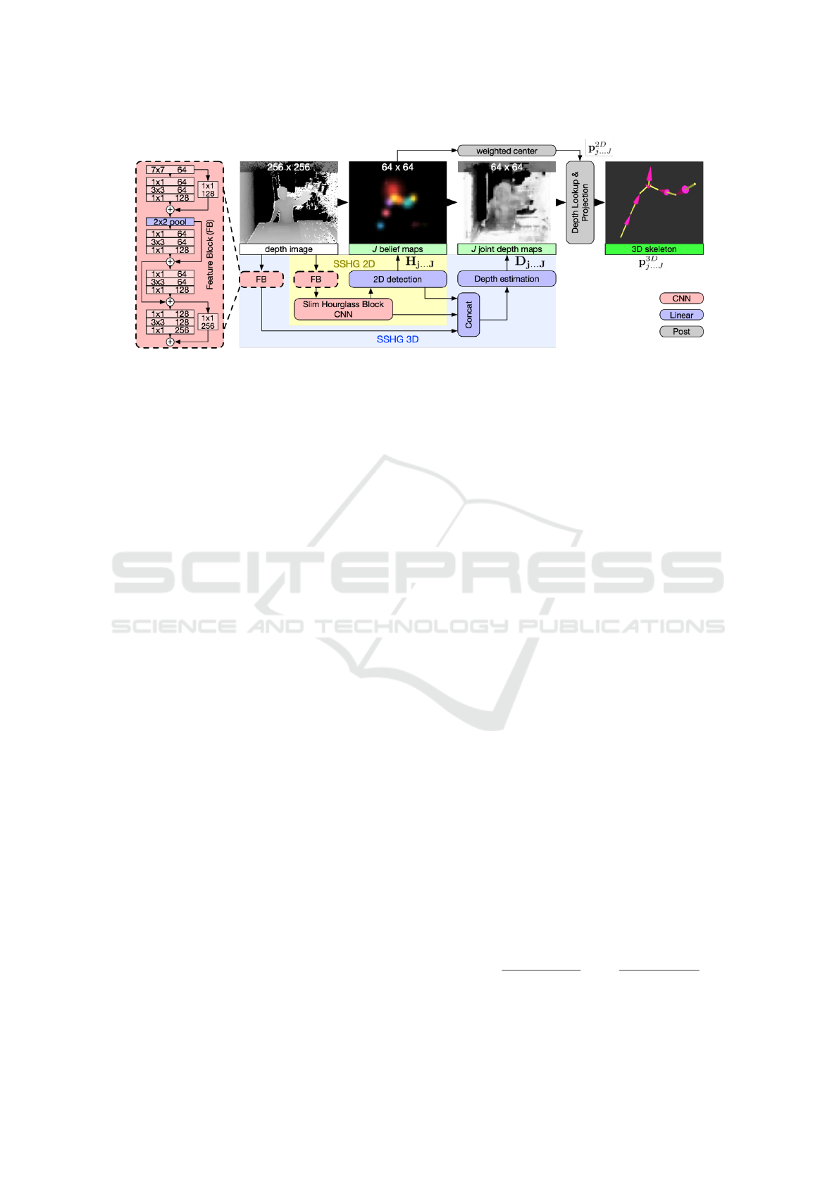
Figure 3: Overview of our 3D pose estimation system: We use four Residual Modules (left) in two separate Feature Blocks
(FB) to compute initial features on the depth image. One Feature Block is used by our Slim Stacked Hourglass CNN (SSHG
2D, see Fig. 2) to produce 2D belief maps H
j
from a single depth image for each upper body joint j. The other Feature Block
is utilized by the second stage which estimates each joint’s distance to the camera with a joint-specific depth map D
j
. The 3D
pose is finally estimated by extracting the 2D location p
2D
j
from H
j
and retrieving the depth from the corresponding depth
map D
j
.
the ten best performing approaches on the MPII Hu-
man Pose Dataset benchmark (Andriluka et al., 2017),
it proved to be well suited for human pose estimation.
Within each Hourglass Block, features are computed
using Residual Modules (Wu et al., 2017) across mul-
tiple scales. By computing features at multiple reso-
lutions and successively combining them, the Stac-
ked Hourglass is essentially a nested multi-resolution
Residual Module. This allows for a large receptive
field while maintaining the ability to consider fine de-
tails. Preliminary to the first Hourglass Block, a Fe-
ature Block like shown in Fig. 3 (left), consisting of
four successive Residual Modules, is used for initial
feature processing. Succeeding the final Hourglass
Block, two linear layers are utilized as a detection
head to produce the final belief maps for each joint.
In our architecture, we make use of the Feature
Block, the Hourglass Block, and the detection head.
Simply put, we wrap an optimized single-stage Stac-
ked Hourglass (SSHG 2D in Fig. 3) with a supple-
mentary Feature Block and detection head to additi-
onally estimate depth maps. While the architecture
of all Feature Blocks and detection heads remains un-
changed, we modify the Hourglass Block for speed
optimization.
3.2 Slim Hourglass Block for Faster
Inference
In order to satisfy our requirement of real-time es-
timation, we optimize the Hourglass Block for our
needs. Several methods for compressing Deep Neural
Networks in order to increase inference speed exist
(Cheng et al., 2017). For simplicity, we choose a va-
riant of weight pruning with successive weight mer-
ging since it can be easily deployed with a low risk of
decreasing performance. Other methods may be still
applied later on for additional speed improvements.
Weight pruning is possible because CNN architec-
tures are often designed generously to prevent bottle-
necks during training. This means that a considerable
amount of weights might waste memory and compu-
ting time even though it does not encode relevant in-
formation that contributes to the inference.
Each convolutional layer takes a multi-channel in-
put and applies a number of filters to produce a multi-
channel output. Since this output is created by mul-
tiplying the layers weights with its input, filters with
weights close to zero can be expected to have no sig-
nificant influence on the output. To determine the mi-
nimum amount of filters necessary to solve the task,
we introduce the measure of channel significance S
c
and filter significance S
f
defined in Eq. 2. They are
based on the normalized cumulative activation A
f ,c
of
a filter patch ~w
f ,c
∈ R
X×Y
across a channel c or filter
f . By computing channel and filter significance for
all layers, we can exclude all weights with a signifi-
cance below a threshold. A visual representation of
the described method for a layer within the Hourglass
Block is shown in Fig. 4.
A
f ,c
= ||~w
f ,c
||
1
=
X
∑
x=1
Y
∑
y=1
|w
x,y
f ,c
| (1)
S
f
=
∑
c
A
f ,c
max
f
0
(
∑
c
A
f
0
,c
)
;S
c
=
∑
f
A
f ,c
max
c
0
(
∑
f
A
f ,c
0
)
(2)
For the Hourglass Block, we were able to remove
VISAPP 2019 - 14th International Conference on Computer Vision Theory and Applications
718

Figure 4: A visual representation of the weights, channel
significance and filter significance for a convolutional layer
taken from a Hourglass Block that was trained on the data
described in Sec. 3.4. This specific layer has 64 input chan-
nels and 64 filters with a 3 × 3 kernel. However, roughly
half of them are not used. a) The value of all weights is co-
lor coded according to the legend on the right. It is easy to
see that a high number of weights is zero and therefore not
used. The activation A
f ,c
of each filter patch ~w
f ,c
∈ R
3×3
is
calculated like described in Eq. 1 and used to determine b)
the channel significance S
c
of each channel and c) filter sig-
nificance S
f
of each filter. By this, channels and filters with
a low significance appear as white horizontal and vertical
gaps respectively. The statistics at the very bottom display
the significance distribution across all channels and filters
which allows to immediately determine the number of used
and unused channels and filters.
more than 55% of the weights across all layers with a
significance threshold of 5%. By this, the number of
parameters was reduced from ≈ 17.4 M to ≈ 7.4 M.
In order to simplify the problem of weight reduction,
the network was trained again afterwards. This way,
it doesn’t matter which specific channels were remo-
ved. By additionally merging all Batch Normalization
layers into the weights of the succeeding convolutio-
nal layers after training (weight merging), the number
of layers was reduced by 51% from 363 to 185. Since
the removed Batch Normalization layers only contai-
ned very few weights, this had no significant impact
on the total number of weights, but reduced the num-
ber of non-parallelizable inference steps.
The resulting architecture reaches the same per-
formance on our task as the original Stacked Hour-
glass, but with only half the number of parameters
and layers. In total, we were able to increase the fra-
merate by about 250% from 17 fps to 58 fps as shown
in Fig. 6 e). This enables real-time pose estimation on
platforms featuring only a single GPU, e.g. , a robot.
3.3 Extension for 3D Estimation
Depth images contain a lot of valuable information
for joint depth estimation (depth meaning distance to
the camera). If the 2D location of all joints is known,
a simple lookup in the depth image might seem like a
sufficient approach. However, depth retrieval still in-
volves three major challenges: First, occlusions (e.g. ,
if the person is holding one hand behind their back)
cannot be resolved directly. Second, noise and low
resolution can introduce large errors for direct depth
lookup, especially for small body parts or great dis-
tances to the camera. This becomes even more proble-
matic, if the 2D joint estimation is not perfect in the
first place. Third, depth images naturally only con-
tain the distance to the body surface. Depending on
the specific joint and pose, estimating the correct dis-
tance to the joint within the body can be difficult.
Some of those problems can be addressed by ad-
ding pre-processing steps on the depth image at the
cost of additional computing time. For example,
successive erosion and dilation can be used to clean
and widen the body silhouette in order to stabilize
the depth lookup. Additionally, depth values may be
averaged in a region around the joint’s location, and a
joint-specific static offset can be used to move a joint
from the surface into the body. We use such an ap-
proach (Fig. 7 a)) as a baseline for comparison. Still,
a lot of inaccuracy and failure cases remain. A more
sophisticated processing pipeline would be necessary
to sufficiently accommodate for occlusions and pose-
specific offsets.
Instead, we extend the Slim Stacked Hourglass
CNN to additionally estimate the depth for each joint.
As shown in Fig. 3, this depth estimation stage con-
sists of two fully connected layers and utilizes the 2D
detection result, the final layer of the Slim Stacked
Hourglass, and an additional Feature Block on the ori-
ginal depth image. In other words, we let the CNN
learn the appropriate depth image pre-processing for
each joint individually. We found the additional Fea-
ture Block to be very benefical for a solid depth esti-
mation.
3.4 Training Data
To capture the specifics of our setup, we created a new
dataset with 150,000 (augmented from 25,000) anno-
tated samples containing 44 motion sequences across
7 categories featuring 5 different actors. Matching our
Real-time 3D Pose Estimation from Single Depth Images
719
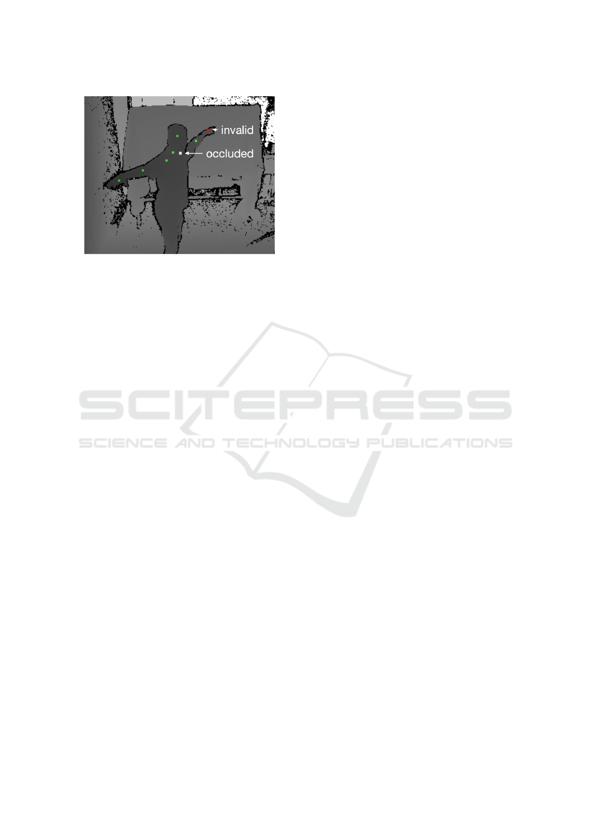
Figure 5: In our training data post processing, labels were
marked as invalid (red) or occluded (white) if their depth
value diverged significantly from the Kinect V2 depth data
(grey).
use case sceanrio, only one actor is present at all ti-
mes. For evaluation, 500 frames of a single unseen
person performing use case actions at the workbench
were recorded.
The recorded sequences are divided into two ca-
tegories, ”work poses” and ”basic poses”. The first
category contains use case movements an the work-
bench such as button interaction, box stacking, key-
board interaction and several idle poses. Using only
this category, many poses (e.g.pointing, walking in
the detection area or having the hands above the head)
would be underrepresented. Therefore, the second ca-
tegory features movements across the hole detection
area with straight or bent arms, pointing and body
touching (which seemed to be especially difficult to
detect correctly). Across all sequences, variations in
background, foreground and actor were introduced.
We created this dataset using the time of flight
depth sensor of a Kinect V2 at 512 × 424 px and the
commercial multi-camera markerless motion tracking
software CapturyLive (Captury Live, 2017) for labe-
ling. Since this method could not produce perfect
labels in every frame, we used a post processing pi-
peline for error detection. There, the label position of
each joint is compared to the depth information cap-
tured by the Kinect V2. As shown in Fig. 5, labels
were marked as invalid or occluded if their depth va-
lue diverged significantly from the Kinect V2 data.
Because all actors were much closer to the camera
than the background, this method reliably differentia-
ted label errors in all axis from occlusions and correct
labels. Only frames with correct labels for all joints
were used for training.
After excluding errors, each of the 25,000 remai-
ning frames was augmented five times by applying
random translations, rotations, and mirroring. For
training, we only considered depth information in a
range range between 0.75 m and 4 m scaled to [0,1].
Also, the input images were rescaled to 256 × 256 to
match the CNN’s input resolution.
3.5 Training
First, we used this dataset to pre-train our Slim
Stacked Hourglass independently for 2D estimation
(SSHG 2D). For this, we generated one belief map
H
GT
j
per joint in which a Gaussian blob denotes the
joint’s 2D position. For this stage, we simply used the
L2 loss.
The whole system (SSHG 3D) was then retrained
for 3D estimation using the same dataset. Here, we
additionally provided one depth map D
GT
j
per joint.
Different to the belief maps H
GT
j
, all pixels of D
GT
j
hold the same value which denotes the joint’s distance
to the camera. Nevertheless, this distance is only con-
sidered at the joint’s actual location during training
by weighting the estimation error (D
j
− D
GT
j
) with
the corresponding ground truth 2D belief map H
GT
j
.
Similar to (Mehta et al., 2017), we defined our depth
loss as
Loss(d
j
) = ||H
GT
j
(D
j
− D
GT
j
)||
2
(3)
where GT indicates the ground truth location and
denotes the Hadamard product.
In both cases, we trained with RMSprop for
200,000 iterations using a learning rate of 2.5×10
−4
,
which is divided by three every 37,500 iterations.
4 RESULTS
We evaluated all results using the PCK
h
(p) measure
(Andriluka et al., 2014) where a joint is considered
detected if the distance between estimated location
and ground-truth is within a fraction p of the head
length. Therefore, this measure can be used for com-
parison across multiple scales in both 2D and 3D. Si-
milar to the state of the art, we define the overall de-
tection rate as PCK
h
(0.5) and the median accuracy (≡
median error) as the normalized distance p
m
where
PCK
h
(p
m
) = 50%.
A comparison on popular datasets like the CMU
Panoptic Dataset (Joo et al., 2015) (used for Open-
Pose) or Human3.6M (Ionescu et al., 2014) would be
desirable but was not possible due to the lack of depth
images or 3D annotations for the depth camera view
point.
VISAPP 2019 - 14th International Conference on Computer Vision Theory and Applications
720
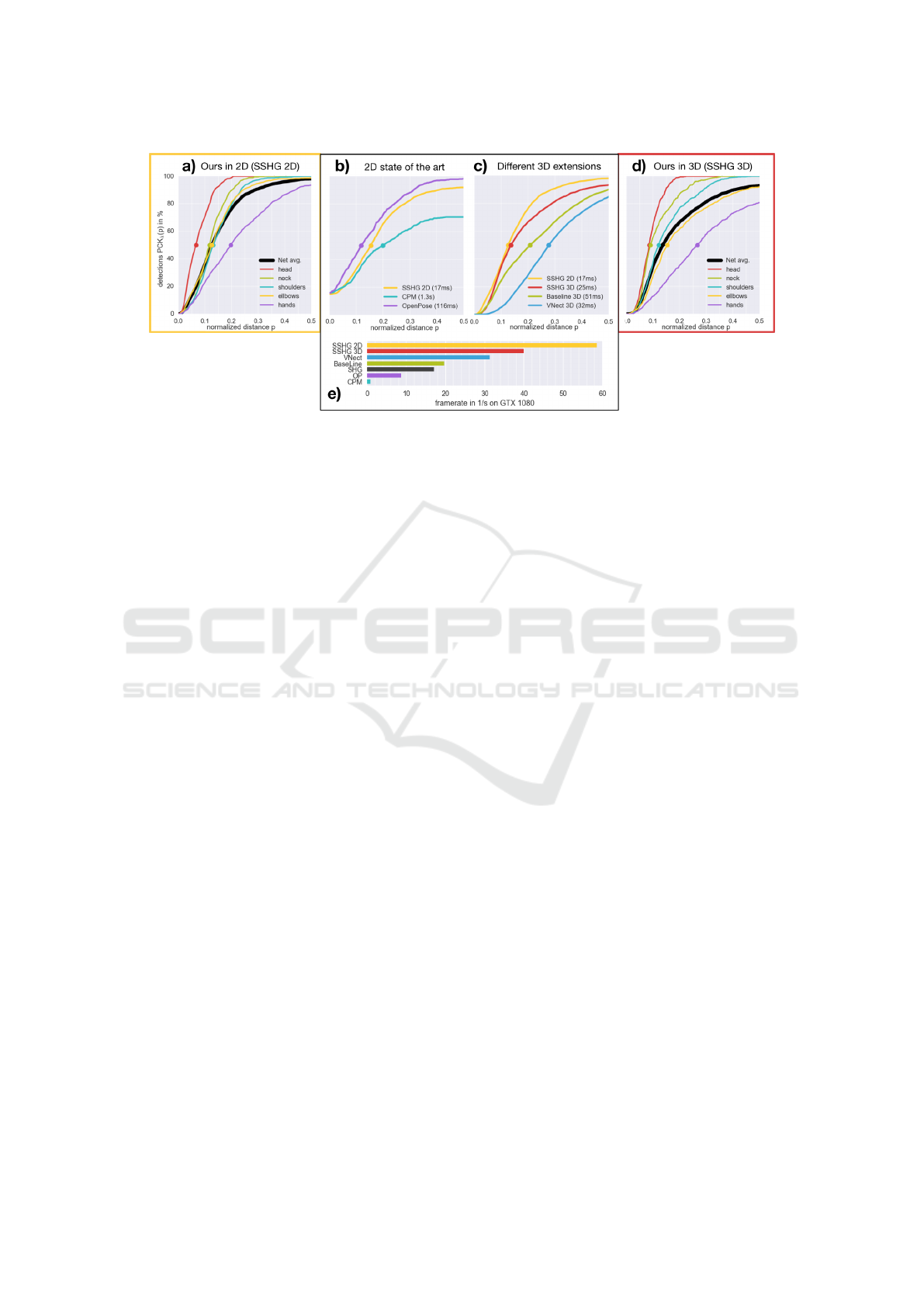
Figure 6: We evaluated the performance of our system by plotting the percentage of correct detections PCK
h
for a maximum
allowed error distance p regarding various aspects (best viewed in color). a) The percentage of correct 2D detections on our
use case evaluation set for all joints. b) Compared with two approaches for 2D estimation, our Slim Stacked Hourglass for
2D estimation almost reaches state of the art accuracy and detection rates. c) Our 3D extension (SSHG 3D) outperforms the
alternative extensions shown in Fig. 7, but does not quite match our 2D performance (SSHG 2D). d) The percentage of correct
3D detections on our use case evaluation set for all joints. e) Our Slim Stacked Hourglass (SSHG 2D) is more than three times
faster than the original Stacked Hourglass (SHG) and five times faster than state of the art approaches (OP, CPM). The final
3D estimation system (SSHG 3D) runs slightly slower due to the additional depth map estimation.
4.1 2D Estimation Performance
Being at the core of our system, we first evaluated the
Slim Stacked Hourglass for 2D joint detection (SSHG
2D). As shown in Fig. 6 a), we achieve a 2D detection
rate of 98% on our use case validation data with a me-
dian error of 0.13 (≈ 2.6 cm). The detection is very
robust for the head with 100% detection rate, but slig-
htly decreases along the kinematic chain. Being at
the end of the kinematic chain, the hands are the most
difficult to detect with a detection rate of 90% and a
median error of 0.2.
To put these results into perspective, we compa-
red our SSHG 2D to two state of the art systems for
2D pose estimation in Fig. 6 b). Since both Open-
Pose (Cao et al., 2017) and the original Convolutional
Pose Machine (Wei et al., 2016) were trained for RGB
images, we created an additional use case validation
dataset for this comparison that includes both depth
and RGB images. While our SSHG 2D was evalua-
ted on the depth images, both state of the art systems
used the corresponding RGB images. Since only visi-
ble joints were labeled in this dataset and the case of
not detecting an occluded joint is counted as an error
of 0, all curves in Fig. 6 b) have an offset at p = 0.
We significantly outperform the detection rate
of the Convolutional Pose Machine which reacted
poorly to the large occlusions caused by the desk.
Even though we do not reach the precision and de-
tection rate of OpenPose entirely, we achieve a com-
parable results at 5 times the speed. Since OpenPose
was trained on a dataset containing 1.5 million fra-
mes and over 500 cameras, we expect the precision
of our system to increase by improving our training
dataset. However, good generalization on a broader
dataset might also require more weights, which might
result in a smaller margin for optimizations like des-
cribed in Sec. 3.2.
4.2 3D Estimation Performance
Based on the results of the SSHG 2D, we compared
three extensions for 3D estimation. The architectures
of all three extensions are shown in Fig. 7 and the cor-
responding 3D estimation performance in Fig. 6 c).
We compared our apprach (Fig. 7 b)) to a more so-
phisticated regression head introduced in VNect (Me-
hta et al., 2017) (Fig. 7 c)) that uses implicit model
knowledge. As a baseline, we additionally implemen-
ted a system that uses a simple lookup (Fig. 7 a)) by
retrieving the joint distance from the original depth
image. To increase precision, we improved this base-
line’s depth image lookup using the post-processing-
steps discussed in Sec. 3.3 at the additional cost of
34 ms.
As evident in Fig. 6 c), our approach outperforms
both alternatives regarding detection rate and accu-
racy while also being the fastest. Most noticeably,
the median detection error increases only marginally
compared to the 2D estimation.
Using this 3D extension approach in the final sy-
stem, the resulting 3D performance on our use case
Real-time 3D Pose Estimation from Single Depth Images
721
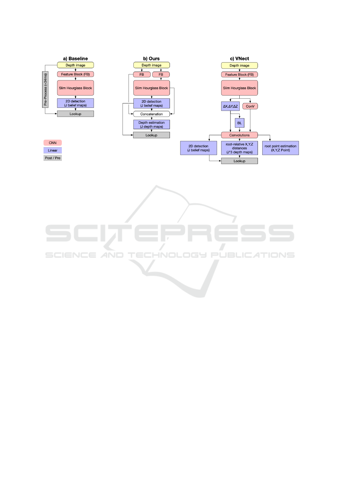
Figure 7: We compare three different architectures to extend our Slim Hourglass Block for 3D estimation. a) A simple lookup
in the original depth image (including pre-processing like described in Sec. 3.3). b) A seperate depth map is estimated for
each joint and used to retrieve the joint depth. c) The VNect regression head (Mehta et al., 2017) combines 2D belief map
prediction with Bone Length estimation (BL), parent-relative distance estimation (∆X, ∆Y, ∆Z) and succeeding root-relative
distance estimation (X,Y,Z) for each joint in all three axis.
validation data is shown in Fig. 6 d) in more detail.
We are able to reach a detection rate of 93% across
all joints with a median error of 0.14 (≈ 2.8cm). The
detection is still very robust for the head, but spreads
out more across the remaining joints. Especially the
performance for hand detection decreases with a de-
tection rate of 80% and a median error of 0.27.
4.3 Limitations
We examined the limitations of our system regarding
multiple aspects. For 3D performance, the quality of
the lookup decreases for persons far away and in noisy
environments. Furthermore, occlusions still cause er-
rors in the depth map lookup. This suggests that our
system only learned to improve the quality of depth
images, but does not contain higher model knowledge
about the human body. Introducing much more occlu-
sions into the training data might improve the perfor-
mance in these situations and force the system to learn
such higher model knowledge. Other than that, the li-
mitations are introduced merely by the 2D estimation
of the Slim Stacked Hourglass.
We found the 2D estimation to be very robust
against the appearance of the subject. All poses in
which the head is visible and at or above shoulder le-
vel can be detected robustly. This corresponds to the
specifics of our training data. Like shown in Fig. 8
a), b), occluded joints other than the head are mostly
detected correctly.
The Slim Stacked Hourglass was trained on a sin-
gle person dataset, but reliably detects multiple pe-
ople as well (Fig. 8 d)). However, the succeeding
system for depth lookup currently works for single
persons only. In order to extend it for multiple per-
sons, an approach for body part association needs to
be implemented. Furthermore, increasing the num-
ber of body joints for detection might also require a
less drastic weight reduction. For full body pose esti-
mation of multiple people, we expect alternatives like
OpenPose to scale better than our system. However,
since this is not necessary in many use cases, we see
the benefits of our approach in scenarios where har-
dware resources are limited and single person pose
estimation is sufficient.
5 CONCLUSION AND FUTURE
WORK
We proposed a system for real-time 3D pose estima-
tion in single depth images that builds upon previous
state of the art approaches. Starting from a single-
stage Stacked Hourglass CNN for 2D pose estimation,
we propose two improvements to create a fast and lig-
htweight 3D estimation architecture. First, a method
for speed optimization was used to reduce both the
amount of parameters and layers by ≈ 50%. By this,
we could increase the speed by a factor of 5 compared
to state of the art systems while maintaining perfor-
mance. Second, an extension for 3D pose estimation
is introduced that addresses the problems of existing
alternatives like a simple lookup or VNect. Our final
system almost matches the 2D performance of much
VISAPP 2019 - 14th International Conference on Computer Vision Theory and Applications
722
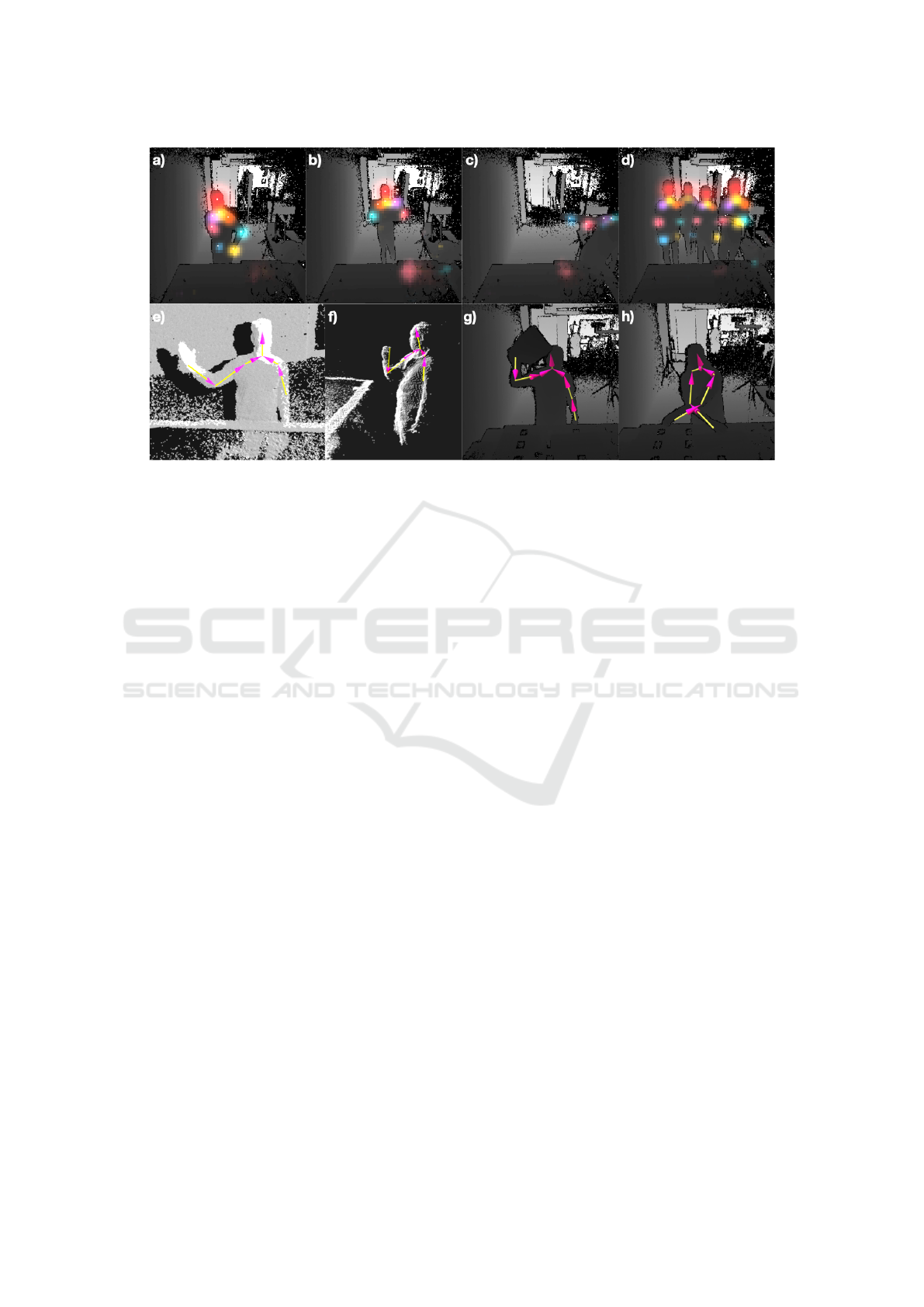
Figure 8: The top row shows some notable aspects of our 2D detection (SSHG 2D) while the bottom row contains examples
for our 3D estmation (SSHG 3D).
a) Minor occlusions (e.g. , a hand behind the back) are mostly detected correctly in 2D. b) Bigger occlusions (e.g. , carrying a
big box in front of the chest) disturb the detection noticeably. This results in a lower accuracy, but does not cause the detection
to fail entirely. c) If the head is occluded (e.g. , outside the frame) or below shoulder height, the detection fails. d) Even
though the system was trained at single person detection only, it correctly detects the 2D location of joints for multiple people.
e), f) Our detection results in 3D overlaid with a point cloud. g) Our detection also works while handling objects. h) Crossing
arms at the workbench is detected correctly.
slower state of the art 2D pose estimation systems and
outperforms alternatives for 3D extensions. We have
successfully deployed the system in our scenario for
Human-Robot-Interaction using the Robot Operating
System ROS. Utilizing the depth sensor of a Kinect
V2, we estimate the 3D position of eight upper body
joints for a single person at up to 40 fps.
For future work, we see two interesting paths. On
one hand, means for improving the performance of
our system may be explored. For example, we expect
our accuracy and detection rate to increase with more
data and higher quality labels. Additionally, a dedi-
cated occlusion data set might force the network to
learn higher model knowledge about the human body
and allow for correct depth retrieval even if joints are
occluded. Both points could also be addressed with a
pipeline for synthetic training data generation.
On the other hand, we see potential for deeper in-
vestigations. This includes analyzing the relations-
hip between the number of reducible weights (as in
Sec.3.2) and other factors, like the number of joints
to be estimated and the size of the training data set.
Also, the possible benefits of using 3D data like depth
images instead of RGB 2D images is an interesting
topic for future research.
REFERENCES
Andriluka, M., Pishchulin, L., Gehler, P., and Schiele, B.
(2014). 2D human pose estimation: New benchmark
and state of the art analysis. In Proceedings of the
IEEE Computer Society Conference on Computer Vi-
sion and Pattern Recognition, pages 3686–3693.
Andriluka, M., Pishchulin, L., Gehler, P., and Schiele, B.
(2017). MPII Human Pose Database Benchmark.
http://human-pose.mpi-inf.mpg.de/#results.
Baak, A., Muller, M., Bharaj, G., Seidel, H. P., and Theo-
balt, C. (2011). A data-driven approach for real-time
full body pose reconstruction from a depth camera. In
Proceedings of the IEEE International Conference on
Computer Vision, pages 1092–1099.
Bulat, A. and Tzimiropoulos, G. (2016). Human pose esti-
mation via convolutional part heatmap regression. In
Lecture Notes in Computer Science (including subse-
ries Lecture Notes in Artificial Intelligence and Lec-
ture Notes in Bioinformatics), volume 9911 LNCS,
pages 717–732.
Cao, Z., Simon, T., Wei, S. E., and Sheikh, Y. (2017). Re-
altime multi-person 2D pose estimation using part af-
finity fields. In Proceedings - 30th IEEE Conference
on Computer Vision and Pattern Recognition, CVPR
2017, volume 2017-Janua, pages 1302–1310.
Captury Live (2017). Captury Live.
http://thecaptury.com/captury-live/.
Cheng, Y., Wang, D., Zhou, P., and Zhang, T. (2017). A
Real-time 3D Pose Estimation from Single Depth Images
723

Survey of Model Compression and Acceleration for
Deep Neural Networks. CoRR.
Chu, X., Yang, W., Ouyang, W., Ma, C., Yuille, A. L., and
Wang, X. (2017). Multi-Context Attention for Human
Pose Estimation. CoRR.
Elhayek, A., De Aguiar, E., Jain, A., Tompson, J., Pishchu-
lin, L., Andriluka, M., Bregler, C., Schiele, B., and
Theobalt, C. (2015). Efficient ConvNet-based marker-
less motion capture in general scenes with a low num-
ber of cameras. In Proceedings of the IEEE Computer
Society Conference on Computer Vision and Pattern
Recognition, volume 07-12-June, pages 3810–3818.
Ionescu, C., Papava, D., Olaru, V., and Sminchisescu, C.
(2014). Human3.6M: Large scale datasets and pre-
dictive methods for 3D human sensing in natural en-
vironments. IEEE Transactions on Pattern Analysis
and Machine Intelligence, 36(7):1325–1339.
Joo, H., Liu, H., Tan, L., Gui, L., Nabbe, B., Matthews, I.,
Kanade, T., Nobuhara, S., and Sheikh, Y. (2015). Pan-
optic studio: A massively multiview system for social
motion capture. Proceedings of the IEEE Internatio-
nal Conference on Computer Vision, 2015 Inter:3334–
3342.
Li, S. and Chan, A. B. (2015). 3D human pose esti-
mation from monocular images with deep convolu-
tional neural network. Lecture Notes in Computer
Science (including subseries Lecture Notes in Artifi-
cial Intelligence and Lecture Notes in Bioinformatics),
9004:332–347.
Martinez, J., Hossain, R., Romero, J., and Little, J. J.
(2017). A simple yet effective baseline for 3d human
pose estimation.
Mehta, D., Sridhar, S., Sotnychenko, O., Rhodin, H.,
Shafiei, M., Seidel, H.-P., Xu, W., Casas, D., and The-
obalt, C. (2017). VNect: Real-time 3D Human Pose
Estimation with a Single RGB Camera. In ACM Tran-
sactions on Graphics, page 14.
Newell, A., Yang, K., and Deng, J. (2016). Stacked Hour-
glass Networks for Human Pose Estimation. Euro-
pean Conference on Computer Vision, pages 483–499.
Rafi, U., Leibe, B., Gall, J., and Kostrikov, I. (2016). An
Efficient Convolutional Network for Human Pose Es-
timation. Procedings of the British Machine Vision
Conference 2016, pages 109.1–109.11.
Shotton, J., Fitzgibbon, A., Cook, M., Sharp, T., Finocchio,
M., Moore, R., Kipman, A., and Blake, A. (2013).
Real-time human pose recognition in parts from single
depth images. Studies in Computational Intelligence,
411:119–135.
Tekin, B., Marquez-Neila, P., Salzmann, M., and Fua, P.
(2017). Learning to Fuse 2D and 3D Image Cues for
Monocular Body Pose Estimation. Proceedings of the
IEEE International Conference on Computer Vision,
2017-October:3961–3970.
Toshev, A. and Szegedy, C. (2013). DeepPose: Human Pose
Estimation via Deep Neural Networks. 2014 IEEE
Conference on Computer Vision and Pattern Recogni-
tion, pages 1653–1660.
Wei, S. E., Ramakrishna, V., Kanade, T., and Sheikh,
Y. (2016). Convolutional pose machines. Pro-
ceedings of the IEEE Computer Society Conference
on Computer Vision and Pattern Recognition, 2016-
December:4724–4732.
Wu, S., Zhong, S., and Liu, Y. (2017). Deep residual lear-
ning for image steganalysis. In Multimedia Tools and
Applications, pages 1–17.
Zhang, L., Sturm, J., Cremers, D., and Lee, D. (2012). Real-
time human motion tracking using multiple depth ca-
meras. Intelligent Robots and Systems (IROS), 2012
IEEE/RSJ International Conference on, pages 2389–
2395.
VISAPP 2019 - 14th International Conference on Computer Vision Theory and Applications
724
