
Trust Dynamics: A Case-study on Railway Sensors
Marcin Lenart
1,2,3
, Andrzej Bielecki
3
, Marie-Jeanne Lesot
2
, Teodora Petrisor
1
and Adrien Revault d’Allonnes
4
1
Thales, Campus Polytechnique, Palaiseau, France
2
Sorbonne Universit
´
e, CNRS, Laboratoire d’Informatique de Paris 6, LIP6, F-75005 Paris, France
3
Student Scientific Association AI LAB, Faculty of Automation, Electrical Engineering,
Computer Science and Biomedical Engineering, AGH University of Science and Technology, Cracow, Poland
4
Universit
´
e Paris 8, LIASD EA 4383, Saint-Denis, France
Keywords:
Trust Dynamics, Trust, Information Quality, Railway Sensors.
Abstract:
Sensors constitute information providers which are subject to imperfections and assessing the quality of their
outputs, in particular the trust that can be put in them, is a crucial task. Indeed, timely recognising a low-trust
sensor output can greatly improve the decision making process at the fusion level, help solving safety issues
and avoiding expensive operations such as either unnecessary or delayed maintenance. In this framework, this
paper considers the question of trust dynamics, i.e. its temporal evolution with respect to the information flow.
The goal is to increase the user understanding of the trust computation model, as well as to give hints about how
to refine the model and set its parameters according to specific needs. Considering a trust computation model
based on three dimensions, namely reliability, likelihood and credibility, the paper proposes a protocol for
the evaluation of the scoring method, in the case when no ground truth is available, using realistic simulated
data to analyse the trust evolution at the local level of a single sensor. After a visual and formal analysis,
the scoring method is applied to real data at a global level to observe interactions and dependencies among
multiple sensors.
1 INTRODUCTION
Information provided by sensors plays a major role
in decision making, especially in automated systems.
Therefore assessing the quality of their outputs, in
particular the trust that can be put in them, is a cru-
cial task. Indeed, there are many situations where
sensors can fail and not produce correct informa-
tion, e.g. due to communication problems, interfer-
ence, difficult operating conditions or calibration is-
sues. Timely recognising untrustworthy information
can increase the usefulness of decision-aid systems,
improve safety and avoid expensive operations such
as either unnecessary or delayed maintenance. To
avoid these issues information can be scored so as to
evaluate its quality level, which is a major topic tack-
led by many authors.
Information Scoring. Information Quality Scoring
has a non-trivial definition for which no consensus
exists, see e.g. (Batini and Scannapieco, 2016). It is
most often decomposed into several dimensions, each
of them focusing on different characteristics of the
considered piece of information, its source or its con-
tent.
An information scoring model can thus be defined
by the individual dimensions it considers and the ag-
gregation procedure used to combine them. More
than 40 different dimensions have been described in
the literature, see e.g. (Sidi et al., 2012). Some ex-
amples for instance include: relevance and truthful-
ness (Pichon et al., 2012); reliability, certainty, cor-
roboration, information obsolescence and source re-
lations (Lesot et al., 2011) or trustworthiness, profi-
ciency, likelihood and credibility (Besombes and Re-
vault d’Allonnes, 2008). Note that a given dimension
name can also have several interpretations and numer-
ical measures to assess them, further enriching the va-
riety of information quality models.
Among the various definitions of information
quality, trust plays a specific role: it interprets the no-
tion of quality as the level of confidence that is put in
a piece of information. As with information quality
scoring in general, existing trust models vary in the
Lenart, M., Bielecki, A., Lesot, M., Petrisor, T. and d’Allonnes, A.
Trust Dynamics: A Case-study on Railway Sensors.
DOI: 10.5220/0007394800470057
In Proceedings of the 8th International Conference on Sensor Networks (SENSORNETS 2019), pages 47-57
ISBN: 978-989-758-355-1
Copyright
c
2019 by SCITEPRESS – Science and Technology Publications, Lda. All rights reserved
47

understanding of the concept it measures and there-
fore in the dimensions used for its representation and
in their aggregation procedure. Some models for in-
stance include confidence, reliability and credibility
(Young and Palmer, 2007); dynamic credibility (Flo-
rea et al., 2010) or reliability, competence, plausibility
and credibility (Revault d’Allonnes and Lesot, 2014).
Information Quality Dimensions for Sensors.
Sensors constitute a specific case of information
providers that are as well subject to imperfections:
they also require to measure the quality of their out-
puts, for instance to allow nuanced processing and
exploitation of their results. Dedicated models have
been developed to take into account their specifici-
ties (Pon and C
´
ardenas, 2005; Guo et al., 2006; Flo-
rea and Boss
´
e, 2009; Destercke et al., 2013; Lenart
et al., 2018). As in the general information quality
case, they are usually defined by a list of individual
dimensions and an aggregation procedure. The most
common dimensions, briefly presented below, are re-
liability, contextual reliability and credibility.
Reliability focuses on the ability of a sensor to
perform its required functions under some stated con-
ditions for a specified time. It is an a priori as-
sessment of the source quality, which can be diffi-
cult to measure. Existing approaches for instance ex-
ploit meta-information about the sensors (Florea and
Boss
´
e, 2009; Destercke et al., 2013) or evaluate its
past accuracy, relying on expert evaluation of its pre-
vious outputs (Florea et al., 2010; Blasch, 2008). The
latter in particular requires the availability of ground
truth to assess the correctness of these previous sensor
outputs.
Contextual reliability adapts reliability depending
on the task the sensor is used for and thus the context
of each piece of information. An example is proposed
in (Mercier et al., 2008) where reliability scoring is
modified to enrich it with its context, thus different
situations can result in different output qualities for a
given sensor. The idea is to create a vector of reliabil-
ity values that are used in different scenarios.
Credibility is usually understood as the level of
confirmation of the considered piece of information
by other, independent, pieces of information. Most
models of credibility can be seen as variations of a
common approach which consists in considering how
many different pieces of information agree with the
evaluated one (Pon and C
´
ardenas, 2005; Guo et al.,
2006; Florea et al., 2010)
This paper considers a specific trust scoring
model, (Lenart et al., 2018), referred to as ReLiC
from hereon and described in Section 2, which relies
on reliability, likelihood and credibility.
Trust Dynamics. There have been several studies
on the issue of trust evolution, examining the succes-
sive values trust can take: trust depends on the in-
formation flow and on the way previous pieces of in-
formation have been scored (Jonker and Treur, 1999;
Falcone and Castelfranchi, 2004; Cvrcek, 2004).
(Jonker and Treur, 1999) argue that a new piece
of information which influences the degree of trust
is either trust-positive, i.e. it increases trust to some
degree, or trust-negative where trust is decreased to
some degree. The degree to which trust is changed
differs depending on the used model. They distin-
guish between two types of trust dynamical models:
a trust evolution function considering all previous in-
formation and a trust update function storing only the
current trust level and having the ability to include
the next information. However, (Falcone and Castel-
franchi, 2004) challenge these definitions, claiming
that this only stands for trust computed as a single di-
mension.
(Mui, 2002) proposes an asymmetrical approach
for the increase/decrease trust rate, which is inspired
by the approach observed in humans: i.e. trust in-
creases slowly but decays rapidly. This asymmetrical
behaviour is also arguably important from a practical
point of view, for many implications (see the case of
malicious attacks in the security domain (Duma et al.,
2005)).
Objectives and Outline. The first goal of this pa-
per is to increase user’s understanding of a dynamic
trust computation model, namely the ReLiC model re-
called in Section 2. ReLiC assesses trust by aggregat-
ing three dimensions, which opens the possibility for
different trust behaviours that highly depend on the
type of quality problem at hand. By analysing these
behaviours it is possible to highlight important trust
evolutions for each encountered problem this show-
ing the user how trust reacts in different scenarios.
Note that, in the expression of trust evolution, trust
is actually successively computed for different pieces
of information and it is not a description of the trust-
worthiness of the source which can be updated by in-
cluding more information. Evolution is understood at
a general level, for the successive messages of a given
sensor.
The second goal is to propose a methodology to
evaluate any quality scoring method, with two im-
portant features. First, the methodology is based on
real data from a given application domain, it is cru-
cial as most of the models are not universal and are
designed only for data from the specific domain in-
cluding specific attributes. Second, contrary to most
related works, this method does not use ground truth
SENSORNETS 2019 - 8th International Conference on Sensor Networks
48

but only statistical properties derived from the data.
This property can be very beneficial as ground truth
is often expensive or impossible to obtain.
Using a visual and formal study of trust be-
haviours we differentiate key trust evolution types that
can occur. We first focus on a controlled evaluation of
the ReLiC method in the case of railway data showing
its capabilities of highlighting possible quality prob-
lems. Then, the method is applied to a real dataset,
named MoTRicS2015 and described in Section 3.2, to
observe the propagation of trust among multiple sen-
sors.
The paper is organised as follows: Section 2 de-
scribes the ReLiC model used in this paper. Sec-
tion 3 presents in more details the proposed method-
ology for trust dynamics evaluation where the con-
ducted studies are divided into the following three
sections: the visualisation of single sensor trust evo-
lution is proposed in Section 4 to evaluate the scoring
method and illustrate its trust evolution, then a formal
analysis is presented on the ReLiC in Section 5. Fi-
nally the real data is used to test the trust propagation
on multiple sensors in Section 6. Section 7 concludes
the paper and discusses future research directions.
2 THE ReLiC MODEL
This section details the information quality model for
sensors (Lenart et al., 2018), from hereon referred to
as ReLiC, on which the study conducted in this paper
is based. ReLiC differs from related work by aiming
to be as self-contained as possible: no ground truth
is needed and all necessary meta-information can be
extracted from the data. Also, the method can be used
in real time as it computes trust dynamically using
only currently available information.
After making explicit the required data structure
and used notations, this section describes in turn each
of the three dimensions as well as their aggregation.
Data Structure. The ReLiC method proposes to
score pieces of information corresponding to sensor
temporal outputs stored as successive log entries for
which the following attributes are available: a date, a
time, a sensor ID and an output message. An example
of the entries from such a log file is given Table 1 (first
four columns) for a single sensor with ID S1, which
outputs two messages: occupied and clear.
In addition, the ReLiC model requires a state tran-
sition graph and a network of sensors. The state tran-
sition graph represents admissible consecutive log en-
tries for one sensor, defining valid transitions: a node
corresponds to the sensor’s output message, an edge
Table 1: Input data structure and output trust scores.
Date Time Sensor ID Message Trust
11.03.2015 07:24:53 S1 occupied 0.9
11.03.2015 07:25:40 S1 occupied 0.3
11.03.2015 08:23:18 S1 occupied 0.7
11.03.2015 08:24:08 S1 clear 0.7
11.03.2015 09:15:23 S1 occupied 0.8
11.03.2015 09:16:08 S1 clear 0.8
11.03.2015 09:39:45 S1 occupied 0.8
11.03.2015 09:40:29 S1 clear 0.8
11.03.2015 10:22:14 S1 occupied 0.8
11.03.2015 10:23:03 S1 clear 0.9
between two nodes indicates that it is possible to have
these two subsequent states (see Section 3.2 and Fig-
ure 2).
The sensor network is a graph whose nodes rep-
resent the sensors and an edge between two nodes in-
dicates that these sensors are correlated, in the sense
that, due to their physical geographical proximity, the
activity of the first one is related to the other one: their
messages are expected to be correlated (see Figure 1).
Notations. Throughout the paper, L denotes the
complete set of log entries and L
s
the set of log en-
tries produced by sensor s. The notation l corre-
sponds to one log entry defined as a vector contain-
ing three values: l.fullDate corresponding to date and
time, l.sensor to the sensor ID and l.message to the
provided piece of information describing the sensor’s
state. The set of all sensors is denoted by S and the
set of all time stamps by T .
Reliability. The first dimension used in the ReLiC
model scores the source independently of its current
message, thus focusing on the specifics of a sensor to
assess an a priori trustworthiness level.
The ReLiC method proposes to consider recent er-
rors produced by the sensor based on the assumption
that an error message suggests a problem with the sen-
sor. Formally, it is defined as:
r : S × T −→ [0, 1]
(s, w) 7−→ 1 −
|error(recent(L
s
, w))|
|recent(L
s
, w)|
(1)
where recent : L × T → P (L) provides the set of the
w latest entries produced by sensor s: w defines a time
window that should depend on the sensor’s output fre-
quency. In the experiments described in Sections 4
and 6, w is set to 20 based on the preliminary exper-
imental studies which consider density of messages.
error : L → P (L ) is the function which extracts the
set of error entries in this set.
Trust Dynamics: A Case-study on Railway Sensors
49

S1 S2 S3 S4 S5
S6 S7 S8 S9
Figure 1: An example of a small sensor network, extracted
from the real data MOTRIcS2015 (see Section 3.2).
Likelihood. The second dimension measures
whether the considered log entry is in line with its
expected possible value, independently of its source,
based on the state transition graph. More precisely,
it examines whether the message flow is compatible
with the model or not. The formal definition of
lkh : L → [0, 1] is:
lkh(l) =
trust(prv(l)), if l.message compatible
with prv(l).message
1 −trust(prv(l)), otherwise
(2)
where prv : L → L returns the single log entry l
0
provided by the same sensor just before the current
entry l and l.message is compatible with l
0
.message
when that state transition exists in the model.
Credibility. The third dimension exploits informa-
tion from other sensors to confirm or deny the consid-
ered entry, also independently of its source. More pre-
cisely, the ReLiC method considers validations and
invalidations taken from the sensor neighbours, where
the neighbourhood is defined by the sensor network,
as illustrated in Figure 1.
Formally, the credibility function cr is defined as:
cr : L −→ [0, 1]
l 7−→ agg
1
(agg
2
(con f (l)), agg
3
(in f (l)))
(3)
where con f : L → P (L) returns a set of entries that
confirm l; in f (l) : L → P (L) returns a set of entries
that contradict l. agg
2
and agg
3
are the aggregation
operators applied to the trust scores of their set of
logs. In (Lenart et al., 2018), they are set to be the av-
erage. The agg
1
operator combines the respective re-
sults provided by agg
2
and agg
3
; (Lenart et al., 2018)
sets it as agg
1
(c, i) =
c+1−i
2
.
Trust. The final step is to aggregate the three pre-
vious dimensions. (Lenart et al., 2018) proposes to
score trust in two steps: it first combines reliability
and likelihood with a conjunctive operator and it then
integrates credibility. The proposed definition is:
tr : L −→ [0, 1]
l 7−→ α ·r(l.sensor, l. f ullDate) · lkl(l)+
(1 −α) · cr(l)
(4)
where the parameter α ∈ [0, 1] weighs the desired in-
fluence of each of the two parts of this equation. In the
experiments described in Sections 4 and 6, α is set to
0.75. The value is proposed in (Lenart et al., 2018)
so as to put more influence on the two dimensions
describing the source and the piece of information it
produces.
As mentioned before, the trust value with its com-
ponents does not depend on a ground truth for an a
priori setup. This separates the ReLiC method from
other approaches taken in the literature.
3 PROPOSED EXPERIMENTAL
METHODOLOGY
This section describes the methodology for the study
of trust dynamics proposed in the paper, discussing
the relevance of data simulation, the considered tools
as well as the proposed experimental protocol applied
to obtain the results presented in Sections 4 and 6.
3.1 Proposed Protocol
The ability to validate a quality scoring method is
a crucial and difficult task as, most often, different
methods use different dimensions which might be
more relevant in one domain and less in other. Usu-
ally, validation is done by using ground truth to com-
pare results provided by the method with the expected
ones. However, the access to ground truth is often dif-
ficult, expensive or sometimes even impossible.
To address this issue, we propose to use realisti-
cally simulated data, based on the real data set we
consider. This approach has two major advantages
apart from making ground truth unnecessary. First,
it gives the ability to create multiple scenarios which
happen rarely in real data or did not happen yet. Sec-
ond, it gives the ability to use data from the same do-
main as the real data which, as mentioned before, is
important with general quality evaluation systems.
Data Simulation. Creating a synthetic database
helps with controlling the type of introduced quality
problems, their intensity, distribution and it allows to
cover a larger spectrum of problems. This opens the
possibility to review different quality problem scenar-
ios to check how the considered method behaves.
SENSORNETS 2019 - 8th International Conference on Sensor Networks
50
We thus propose to create a synthetic log entries
set by randomly modifying a certain amount of origi-
nal entries, to introduce quality problems in the data.
The modifications consist in replacing the message
that an entry carries with a different one in the pos-
sible set of messages thus creating a noisy dataset.
Then, the original data serves as a ground truth for
future validation.
For a given set of log entries, the simulation mod-
ifies a certain percentage of the entries produced by a
sensor with different distributions.
Analysis Methodology. The analysis of trust dy-
namics consists in studying the difference between
two consecutive trust values, which we denote
∆(tr) = trust
2
− trust
1
in the following. By intro-
ducing noise to one of the sensors we can study how
∆(trust) changes as well as ∆(r), ∆(lkl) and ∆(cr).
First, a visual analysis of local dynamics considers
the level of decrease in simulated entries and its later
recovery to observe the effectiveness of the ReLiC
method in recognising quality problems and to illus-
trate its trust evolution behaviours in these situations
in Section 4. Then, a formal study of the formulas
used to score each dimension is performed to observe
theoretical dependencies and explain previously ob-
served behaviours in Section 5.
Finally, the ReLiC method is used to compute
trust for real data and to observe the global trust dy-
namics of information from multiple sensors interact-
ing with each other in Section 6. A new visualisation
scheme is proposed for plotting the trust evolution for
all available sensors simultaneously. This can easily
show how neighbouring sensors can influence each
other.
The presented method as well as the proposed
experimental methodology apply to any information
produced by event-based sensors, even though this
study focuses on railway data.
3.2 The MoTRicS2015 Real Data
Data Presentation. In this paper we consider a
dataset called MoTRicS2015 which stems from the
rail signalling domain and incorporates different
kinds of monitoring devices such as axle counters or
point machines. It consists of entries which store the
information about asynchronous events produced by
the devices located on the railway tracks. We consider
one of the stations covered in MoTRicS2015 and its
surrounding tracks for one year of available data. In
the experiments, only one type of sensor is evaluated,
the axle counter (AC). This device provides informa-
tion about a train entering a specific part of track or
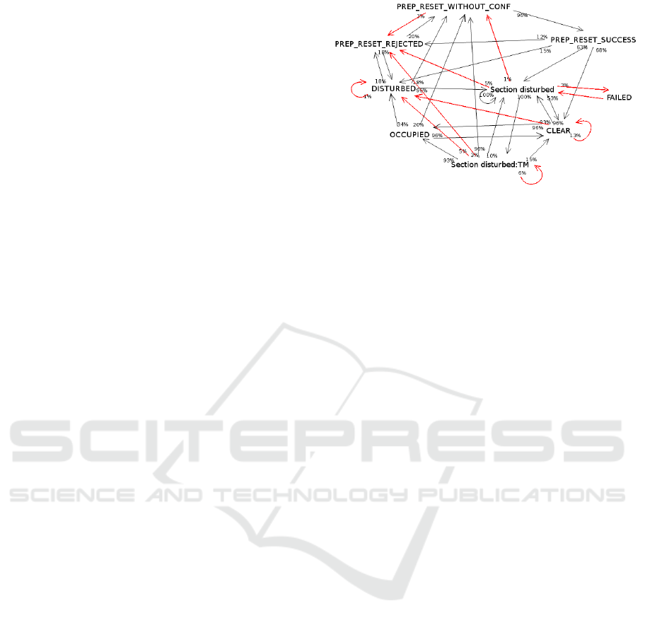
Figure 2: State transition graph, extracted from the real data
MoTRicS2015 (see Section 3.2).
leaving it. It constitutes an event-based type of infor-
mation. Multiple devices of this type show the move-
ment of a train and are needed for safety passage.
In the considered part of the railway there are 60
AC providing 1,142,302 log entries within one year
time.
State Transition Graph Extraction. In the ab-
sence of a theoretical model we propose to build the
state transition graph automatically from the data.
First, for each AC, its log entries are extracted and
their unique messages are used as nodes in a graph.
The transition between two nodes is created if the
two subsequent messages can be found in the anal-
ysed entries. This transition graph is created for ev-
ery AC in the data thus amounting to 60 such graphs.
Next, they are aggregated into a global graph with
the aim of keeping a maximum number of nodes and
transitions. Each transition is weighted by the pro-
portion of AC that have this transition (the percent-
ages shown in Figure 2). Some connections above
the threshold were removed when their temporal fre-
quency (percentage of occurencies per AC) is below
a given threshold of 10%.
The result of this data extraction is shown in Fig-
ure 2, where the red connections are the removed
ones. The main nodes indicate that a train entered the
track section (occupied), a train left the track section
(clear) or different error states (the other messages).
4 ILLUSTRATIVE EXAMPLE
This section analyses the trust evolution at a local
level, when a single sensor has quality problems. It
analyses the visual representation of its trust evolu-
tion, in particular different types of trust decreases as
well as the later increases leading to get back to the
previous trust degree, called recovery.
Trust Dynamics: A Case-study on Railway Sensors
51

Two noise distributions are considered: in the first
case, noise is uniformly distributed in the whole pe-
riod; in the second case, burst noise is considered, i.e.
noise concentrated within a short time period. To il-
lustrate the results, the first case is denoted as C1 and
the second as C2.
4.1 Considered Visualisation
By altering the original data we can observe how the
trust value evolves for a given sensor. It is possible to
analyse not only the level of decrease but also what
happens immediately after trust decreases in a simu-
lated entry.
Figures 3 to 10 present the trust evolution over
time, as well as the evolution of the three considered
dimensions. Fig. 3 to 6 correspond to the uniform
noise distribution, Fig. 7 to 10 the concentrated one.
The trust evolution is shown on Fig. 3 and 7, reliabil-
ity on Fig. 4 and 8, likelihood on Fig. 5 and 9 and
credibility on Fig. 6 and 10.
In each graph, the x-axis represents time measured
as the log entry number, the y-axis represents the con-
sidered dimension (trust, reliability, likelihood and
credibility). The graphs only show the noisy sensor,
all the others in the data set being left intact and hav-
ing a trust value of 1 over the considered interval.
A simulated entry change is highlighted by a ver-
tical line. Additional information about the applied
modification is provided by the line colour:
• blue: occupied modified to clear
• orange: occupied modified to one of the error
states
• violet: clear modified to occupied
• green: clear modified to one of the error states
Note that, for the analysis, not all of the error states
are considered when introducing noise, but only two
of the most common ones.
4.2 Observations
This section comments the trust evolution and then of
its components: reliability, likelihood and credibility.
Trust. The first important observation is that all si-
mulated entries indeed have a decreased trust value,
which is a first validation of the proposed method. A
clear example of this decrease is provided by case C1,
entry 146: it illustrates the level of single decrease
for a non-error noise and the recovery taking place
afterwards, where trust increases but not instantly.
This behaviour is desired (see Section 1), where the
trust evolution patterns are asymmetrical, with fast
decreases and slow recoveries.
We can observe that the amplitude can vary, up to
−0.92 (C1, entry 95) followed by a quick recovery
next (∆(tr) = 0.83). In the case of denser noise, more
fluctuations can be observed comparing to the noise
distributed more sparsely (entries 8-54, C1). This be-
haviour is further studied with the burst noise trust
evolution illustrated in graphs 7-10.
Here, an interesting fact can be highlighted: as in
C1 (entries 90-105) the trust level highly fluctuates
differentiating the noisy parts from the unchanged en-
tries. This shows that even in the dense noise sce-
nario the ReLiC method can successfully find the pe-
riods where the sensor works properly. Again, trust
can quickly recover thanks to credibility which is very
high since all neighbouring sensors are working cor-
rectly and are able to confirm the correct message.
Reliability. Figures 4 and 8 show the evolution of
reliability. As expected, reliability decreases after
simulated error-type entries (orange and green lines)
and this decrease remains for 20 entries, which is in
line with the window parameter of the recent func-
tion (see Equation 1). Note that in the considered
part of data, there is no simulated error messages. We
can observe a “stair-like” behaviour where reliability
encounters another error entry or recovers from one.
Other types of entry modifications (blue and violet)
do not impact reliability in any way, as expected.
Likelihood. Figures 5 and 9 show the evolution of
likelihood. We can observe that, for C1, its shape is
highly similar to that of trust, with a very small de-
lay of one time stamp: the simulated entries appear
to be usually compatible with the previous messages,
making the likelihood equal to the trust value of the
previous message (see Equation 2). However, this is
not the case with the concentrated noise represented
in C2, where compatibility is not observed anymore,
leading to more contrasted behaviours.
These figures also illustrate the case where noise
does not break the possible sequence of messages
with the previous entry and does not contribute to
lowering the trust value (e.g. entry 9 in C1). How-
ever it disrupts the next entry as there is no connec-
tion from the noisy message to the normal one. It is
observed here as a likelihood decrease after the high-
lighted noise (e.g. entries 11 or 155 in C1). That can
also be the cause, apart from reliability, to further de-
crease trust instead of recovering it.
Credibility. The two examples of credibility evolu-
tion are illustrated in Figures 6 and 10. Most of the
SENSORNETS 2019 - 8th International Conference on Sensor Networks
52
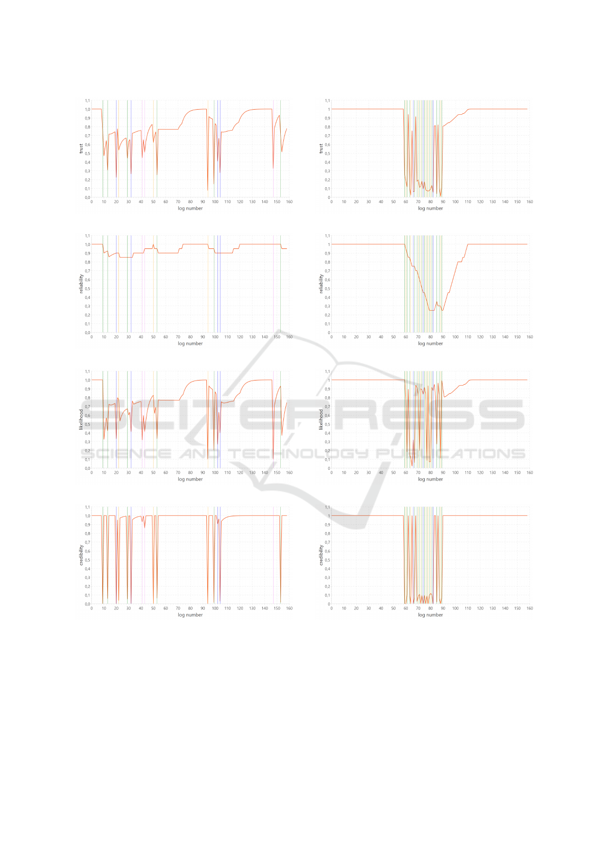
Figure 3: C1, uniform noise distribution: trust.
Figure 4: C1, uniform noise distribution: reliability.
Figure 5: C1, uniform noise distribution: likelihood.
Figure 6: C1, uniform noise distribution: credibility.
time, credibility stays close to 1 or 0. As already
stated, in this local level study, a single sensor has
noisy entries, the neighbouring sensors do not have
modified entries. Therefore, their trust is usually close
to 1. This causes such an instant decrease in credibil-
ity in short time. This behaviour is especially high-
lighted in C2 where credibility is instantly high when
the message is not simulated even though it is in the
Figure 7: C2, concentrated noise distribution: trust.
Figure 8: C2, concentrated noise distribution: reliability.
Figure 9: C2, concentrated noise distribution: likelihood.
Figure 10: C2, concentrated noise distribution: credibility.
middle of high dense noise.
However we can observe that credibility is not af-
fected by one of the modification types or it is in small
level, i.e. the change from clear to occupied, repre-
sented by the violet line (e.g. entry 146 in C1). This
behaviour is strange as this only happens in clear to
occupied transition and does not in occupied to clear.
It is caused by an improper confirmation recognition
Trust Dynamics: A Case-study on Railway Sensors
53

made possible due to the fact that occupied state is
produced shortly before clear.
5 FORMAL STUDY OF THE
TRUST EVOLUTION
This section analyses the trust behaviour by studying
the equations defining each dimension, as well as the
final aggregation into the trust value. By analysing
each dimension separately, we want to emphasise the
extent of their ability to modify trust over time. In ad-
dition, by combining the analysis of each dimension,
we investigate the largest possible trust decrease.
In the following, the notion of ∆(trust) is com-
puted as a difference between the trust value of the
current sensor output trust(r
2
, lkl
2
, c
2
) and the trust
value of the previous sensor output trust(r
1
, lkl
1
, c
1
)
which shows the level of decrease or recovery for
trust. Formally it is then:
∆(trust) = trust(r
2
, lkl
2
, c
2
) − trust(r
1
, lkl
1
, c
1
)
= α ·r
2
· lkl
2
+ (1 −α) · c
2
− (α ·r
1
· lkl
1
+ (1 −α) · c
1
)
where α ∈ [0, 1] and reliability depends on fixed win-
dow of w > 0 previous entries (see Section 2).
Reliability Analysis. Let us consider the influence
of reliability independently of other dimensions by
making lkl and c constants, then:
∆(trust) = trust(r
2
, lkl, c) −trust(r
1
, lkl, c)
= α ·lkl · (r
2
− r
1
)
= α ·lkl · ∆(r)
i.e. the evolution of trust is expressed as the level of
reliability change multiplied by α · lkl. Therefore, re-
liability has the biggest impact when likelihood is set
to its maximum value, lkl = 1.
Reliability strongly depends on the “recent” func-
tion which returns w previous entries of the same sen-
sor. Within those w entries we denote the number of
error entries e and regular entries m, e+m = w. When
considering the next entry we discard the oldest one.
This gives us two possibilities, if both entries belong
to the same group (error or regular), then the change
in reliability is 0, ∆(r) = 0. If they belong to different
groups, we have two possibilities as well: either the
latest entry is an error (m decreases and e increases
by 1) or it is a regular message (m increases and e
decreases by 1), in that case, the change in reliability
can be a decrease:
∆(r) =
w −(e + 1)
w
−
w −e
w
= −
1
w
or recovery:
∆(r) =
w −(e − 1)
w
−
w −e
w
=
1
w
Considering this behaviour of reliability and by
setting constant lkl = 1, we can narrow the possible
trust evolution to three values:
∆(trust) ∈
−α ·
1
w
, 0, α ·
1
w
We can notice only one decrease and recovery
level for reliability, that explains the previously de-
scribed behaviour in Figures 4 and 8 where the relia-
bility evolution has a stair-like behaviour.
Likelihood Analysis. To study the influence of
likelihood on trust, let us consider r and c as con-
stants, then:
∆(trust) = trust(r, lkl
2
, c) −trust(r, lkl
1
, c)
= α ·r · (lkl
2
− lkl
1
)
= α ·r · ∆(lkl)
Again, we can observe that the trust evolution is pro-
portional to likelihood, with multiplicative factor α ·r,
which means that the biggest decrease happens with r
as maximum value, r = 1.
Even though there are no dependencies from the
previous likelihood value to the current one, we can
highlight some interesting properties. Let us consider
three consecutive entries l
0
, l
1
and l
2
with constant
reliability and credibility where either both transitions
are valid according to the considered state transition
graph or not.
In the first case, according to the ReLiC model,
lkl(l
1
) = trust(l
0
) and lkl(l
2
) = trust(l
1
), which leads
to
∆
2
(trust) = tr(l
2
) − tr(l
1
) = α · r · (lkl
2
− lkl
1
)
= α ·r · (tr(l
1
) − tr(l
0
)) = α · r · ∆
1
(trust)
Thus we can observe that if the information flow ap-
pears as likely, then trust continues its previous de-
crease or recovery multiplied by α · r. Since α ∈ [0, 1]
and r ∈ [0, 1], that makes each following decrease or
recovery equal or slower: |∆
n
(trust)| 6 |∆
n−1
(trust)|.
On the other hand, when the two consecutive
pieces of information are not compatible with the
model, lkl(l
1
) = 1 − trust(l
0
) and lkl(l
2
) = 1 −
trust(l
1
), leading to
∆
2
(trust) = −α · r · ∆
1
(trust)
We can see that in a case where pieces of informa-
tion are considered as unlikely, likelihood reverses the
trend of trust, changing decreasing to recovery and
vice versa. This observation shows that in continuous
quality problems, detected by likelihood, a fluctua-
tion behaviour can be observed, where the trust evolu-
tion can consist in alternated decreases and increases.
Again, since it is multiplied by α · r, where α ∈ [0, 1]
SENSORNETS 2019 - 8th International Conference on Sensor Networks
54

and r ∈ [0, 1], |∆
2
(trust)| 6 |∆
1
(trust)| which creates
the oscillation of equal or decreasing magnitude. This
type of behaviour was indeed observed in Figure 3
(see Section 4.2).
Credibility Analysis. The credibility dimension is
defined independently from the previous two dimen-
sions and its scoring is based entirely on the compar-
ison of the considered piece of information with the
ones provided by different sensors. When consider-
ing r and lkl as constant, it holds that
∆(trust) = trust(r, lkl, c
2
) −trust(r, lkl, c
1
)
= (1 −α) · (c
2
− c
1
)
= (1 −α) · ∆(c)
We can notice that constant r and lkl are irrelevant
when analysing the impact of credibility on trust dif-
ference. The evolution of trust is proportional to cred-
ibility’s, with multiplicative factor (1 − α). However,
there is no correlation between the previous credibil-
ity value and the current one, nor with any previous
dimension. This can be observed by analysing credi-
bility’s formula which only aggregates messages from
other sources. Therefore ∆(c) is only limited by cred-
ibility value itself which is in [0, 1] range. Then, by
including (1 − α) factor, the possible trust evolution:
∆(trust) ∈ [α − 1, 1 − α].
6 TRUST DYNAMICS OF
MULTIPLE SENSORS IN REAL
DATA
The analysis from the previous sections shows the
ability of the ReLiC method to highlight possible
quality problems at a local level (single sensor). In
this section we analyse the global behaviour of the
trust evolution and how different trust levels impact
other sensors based on the MoTRicS2015 real dataset
from railway domain (see Section 3.2). Indeed, the
ReLiC method gives an opportunity to observe how
a sudden decrease in trust for one sensor can im-
pact other ones and their trust computation. However,
to observe this possible propagation to neighbouring
sensors, we need a way to illustrate trust level for all
sensors in one chart.
In the following we describe our approach to il-
lustrate results provided by all sensors at once in Sec-
tion 6.1 to later use it as a tool to analyse and interpret
the results in Section 6.2.
6.1 Proposed Visualisation
The trust values are computed for the 60 axle coun-
ters, each having around 25 000 entries in the dataset
(see Section 3.2). In order to compare the trust dy-
namics for all of them we propose the following RGB
visualisation.
RGB Chart. The chart uses time on the x-axis and a
sensor ID on the y-axis. Using time instead of an entry
line number in the x-axis allows an easy comparison
of trust values between multiple sensors. The trust
values are represented by a colour between yellow,
representing the highest trust, and red representing the
lowest trust. White spaces indicate the lack of entries
within that time for the corresponding line.
Trust Temporal Aggregation. The trust values
presented in the chart are aggregated within an a pri-
ori specified time window t. A higher t allows to dis-
play a bigger time frame, however a lower t displays
a more detailed view.
In MoTRicS2015, sensors produce a low number
of entries per hour which makes t = 1h a good com-
promise between displaying a large time frame and
important details.
A conjunctive behaviour is desired for this aggre-
gation operator. Indeed we want to strongly highlight
the decrease in trust value within the data. The cur-
rently proposed function is the minimum, which pri-
oritises the lowest trust value.
The procedure for visualising trust values as an
RGB chart is as follows: entries produced by the same
sensor are grouped together. For each group, trust val-
ues within the same hour are aggregated to create a
pair (d, tr), where d is a date and hour for this aggre-
gation and tr is an aggregated trust value. Each trust
value is then translated to a colour between red and
yellow. Then, for each group, their pairs are plotted
in the RGB chart.
Sensor Order. The order of the displayed sensors
is another issue. One possibility is to choose the first
sensor and use for the next one its neighbour. This
gives an opportunity to observe a behaviour which af-
fects multiple neighbouring sensors.
All 60 sensors can be divided into three groups.
The first two represent ACs in the same set of tracks,
for trains going in each direction, the third set con-
tains the rest which mostly corresponds to backup
tracks on the platform. To keep an understandable
quantity of data, these backup sensors are omitted
for simplicity in this study, the remaining ones cor-
respond to 39 sensors in total.
Trust Dynamics: A Case-study on Railway Sensors
55

Figure 11: Trust value evolution for 39 sensors of the real
data MOTRIcS2015.
Figure 11 shows the obtained results, the thicker
black line indicates that two sensors are not neigh-
bours. The chart width is limited to 3000 hours which
corresponds to approximately 4 months out of 1 year
available data.
6.2 Results
We can first observe that sensors do not report activity
all the time, there are hours where there is lack of any
activity for numerous sensors showed as white spaces.
We can also see that even though the beginning of
the chart looks trustworthy, some major quality prob-
lems are later encountered, visualised as low trust in-
formation across multiple sensors (groups A and B)
which are further discussed below. In addition, we
can notice multiple smaller sites where the trust value
is low (e.g. C group), this behaviour is analysed later.
Global Issues. Different problems with readings
from sensors can be caused by external sources, for
instance, power outages, software updates or global
system failures. Usually that kind of problems can be
observed for many sensors at the same time.
In Figure 11, the A & B groups of trust decreases
are similar for many sensors in the same time. Such
a behaviour can indeed indicate some external prob-
lems which influence many neighbouring sensors at
the same time and raise alerts for a domain expert.
Trust Decrease Propagation. The analysis of the
dynamic trust scoring method shows its dependency
on other sources scored by the credibility dimension
(see Section 2). In the considered AC case, the credi-
bility score directly depends on the trust value of one
of its neighbours. By defining confirming and con-
tradicting information, the neighbouring sensors have
an impact to the trust of the evaluated log entry which
can be increased or decreased. As shown in Section
Figure 12: Trust decrease propagation to multiple sensors.
4, the sensor can provide low trust message due to
some quality issues, thus starting a phenomenon of
low trust propagation among neighbours. Figure 12
presents the enlarged version of the C portion in Fig-
ure 11, where an important trust decrease occurs in
one of the sensors.
This visualisation shows that the low-trust in this
sensor messages, as expected, affects the neighbour-
ing ones in this time window. The reason for this is
that the initial trust decrease disrupts a further chain
of confirmations. The neighbour either lacks the ex-
pected confirming entry or has to consider a low-trust
one. In either case, it causes the propagation of trust
decrease to the neighbouring sensor. The level of trust
decrease is lesser in each new sensor. The difference
is controlled by the a priori set α value (see Equa-
tion 4). By manipulating this constant, it is possible to
change the level of low trust propagation to the neigh-
bour, which also affects the number of sensors that are
affected by the original trust decrease.
In Figure 11 we can observe many similar sin-
gle trust decreases. As this dataset was not prepro-
cessed by an expert, its quality is unknown before-
hand and possible quality problems can be encoun-
tered. While most of the time trust is high on this
dataset, our method points out several low-trust en-
tries. This can be used as an alert procedure for the
operational system indicating a drift in quality either
in the data collection process (data loggers) or the sen-
sors themselves.
7 CONCLUSION AND
PERSPECTIVES
Understanding the process of trust assessment is a
much needed feature for a sensor-based decision-
aid system: low-trust sensor information may be ex-
cluded from fusion or maintenance scheduling, but
this is conditioned by the validation of the scoring
as well. This can be tackled by studying the dynam-
ics of trust over time for a single sensor, as well as
for multiple sensors simultaneously. In this paper we
SENSORNETS 2019 - 8th International Conference on Sensor Networks
56

have analysed this dynamics in a three-dimensional
scoring framework, where the contributions of each
independent dimension to the global trust score were
considered, both at formal and experimental levels.
We proposed a methodology based on simulated data,
obtained by noise injection in real data which makes
it possible to perform an experimental study of the
considered trust model in the absence of an available
ground truth for the real data. We have shown that the
expected evolution of trust based on its definition in-
deed occurs when different types of faulty messages
are injected in the data. Moreover, we have experi-
mentally illustrated the propagation of trust decreases
in a network of neighbouring sensors on a real-world
dataset without ground truth. Future work includes
field-expert validation of the models extracted from
the data as well as the usability of the different ob-
tained trust levels and recovery delays.
REFERENCES
Batini, C. and Scannapieco, M. (2016). Data and Informa-
tion Quality. Springer International Publishing.
Besombes, J. and Revault d’Allonnes, A. (2008). An exten-
sion of STANAG2022 for information scoring. In Int.
Conf. on Information Fusion, FUSION’08, pages 1–7.
Blasch, E. (2008). Derivation of a reliability metric
for fused data decision making. In IEEE National
Aerospace and Electronics Conference, pages 273–
280.
Cvrcek, D. (2004). Dynamics of reputation. In 9th Nordic
Workshop on Secure IT-systems (Nordsec04), pages
1–14.
Destercke, S., Buche, P., and Charnomordic, B. (2013).
Evaluating data reliability: An evidential answer with
application to a web-enabled data warehouse. IEEE
Trans. Knowl. Data Eng., 25(1):92–105.
Duma, C., Shahmehri, N., and Caronni, G. (2005). Dy-
namic trust metrics for peer-to-peer systems. In Proc.
of the 16th Int. Workshop on Database and Expert Sys-
tems Applications, pages 776–781. IEEE.
Falcone, R. and Castelfranchi, C. (2004). Trust dynamics:
How trust is influenced by direct experiences and by
trust itself. In Proc. of the 3rd Int. Joint Conf. on
Autonomus Agents and Multiagent Systems (AAMAS
2004), pages 740–747. IEEE.
Florea, M. C. and Boss
´
e,
´
E. (2009). Dempster-Shafer
Theory: combination of information using contextual
knowledge. In Int. Conf. on Information Fusion, FU-
SION’09, pages 522–528. IEEE.
Florea, M. C., Jousselme, A.-L., and Boss
´
e,
´
E. (2010). Dy-
namic estimation of evidence discounting rates based
on information credibility. RAIRO-Operations Re-
search, 44(4):285–306.
Guo, H., Shi, W., and Deng, Y. (2006). Evaluating sen-
sor reliability in classification problems based on evi-
dence theory. IEEE Trans. on Systems, Man, and Cy-
bernetics, Part B (Cybernetics), 36(5):970–981.
Jonker, C. M. and Treur, J. (1999). Formal analysis of
models for the dynamics of trust based on experi-
ences. In European Workshop on Modelling Au-
tonomous Agents in a Multi-Agent World, pages 221–
231. Springer.
Lenart, M., Bielecki, A., Lesot, M.-J., Petrisor, T., and
d’Allonnes, A. R. (2018). Dynamic trust scoring of
railway sensor information. In International Confer-
ence on Artificial Intelligence and Soft Computing,
pages 579–591. Springer.
Lesot, M.-J., Delavallade, T., Pichon, F., Akdag, H.,
Bouchon-Meunier, B., and Capet, P. (2011). Propo-
sition of a semi-automatic possibilistic information
scoring process. In Procs. of the 7th Conf. of the
European Society for Fuzzy Logic and Technology
(EUSFLAT-2011) and LFA-2011, pages 949–956. At-
lantis Press.
Mercier, D., Quost, B., and Denœux, T. (2008). Refined
modeling of sensor reliability in the belief function
framework using contextual discounting. Information
Fusion, 9(2):246–258.
Mui, L. (2002). Computational models of trust and rep-
utation: Agents, evolutionary games, and social net-
works. PhD thesis, MIT.
Pichon, F., Dubois, D., and Denoeux, T. (2012). Relevance
and truthfulness in information correction and fusion.
Int. Jour. of Approximate Reasoning, 53(2):159 – 175.
Pon, R. K. and C
´
ardenas, A. F. (2005). Data quality infer-
ence. In Proc. of the 2nd Int. Workshop on Information
quality in information systems, pages 105–111. ACM.
Revault d’Allonnes, A. and Lesot, M.-J. (2014). Formalis-
ing information scoring in a multivalued logic frame-
work. In Proc. of the 15th Int. Conf. on Informa-
tion Processing and Management of Uncertainty in
Knowledge-Based Systems, (IPMU 14). Part I, pages
314–324. Springer.
Sidi, F., Panahy, P. H. S., Affendey, L. S., Jabar, M. A.,
Ibrahim, H., and Mustapha, A. (2012). Data quality:
A survey of data quality dimensions. In Proc. of Int.
Conf. on Information Retrieval Knowledge Manage-
ment, pages 300–304.
Young, S. and Palmer, J. (2007). Pedigree and confidence:
Issues in data credibility and reliability. In Int. Conf.
on Information Fusion, FUSION’07.
Trust Dynamics: A Case-study on Railway Sensors
57
