CollabNet - Collaborative Deep Learning Network

Mois

es Laurence de Freitas Lima Junior

, Will Ribamar Mendes Almeida

and Areolino de Almeida Neto

Department of Computing, Federal Institute of Tocantins (IFTO), Village Santa Teresa - km 06, Araguatins-TO, Brazil

Department of Computing, CEUMA University (UNICEUMA), Rua Josu

e Montello - 1, S

ao Luis-MA, Brazil

MecaNET group, Federal University of Maranhao (UFMA), Av. dos Portugueses - 1966, Sao Luis-MA, Brazil

Keywords:

Deep Learning, Deep FeedForward, Deep Stacked Autoencoder.

Abstract:

The goal is an improvement on learning of deep neural networks. This improvement is here called the Col-

labNet network, which consists of a new method of insertion of new layers hidden in deep feedforward neural

networks, changing the traditional way of stacking autoencoders. The new form of insertion is considered

collaborative and seeks to improve the training against approaches based on stacked autoencoders. In this new

approach, the addition of a new layer is carried out in a coordinated and gradual way, keeping under the control

of the designer the inﬂuence of this new layer in training and no longer in a random and stochastic way as

in the traditional stacking. The collaboration proposed in this work consists of making the learning of newly

inserted layer continuing the learning obtained from previous layers, without prejudice to the global learning

of the network. In this way, the freshly added layer collaborates with the previous layers and the set works in a

way more aligned to the learning. CollabNet has been tested in the Wisconsin Breast Cancer Dataset database,

obtaining a satisfactory and promising result.

1 INTRODUCTION

The use of machine learning techniques is becoming

more frequent in the most varied tasks of everyday

life, and the growth of this area of knowledge con-

tinues at a fast pace. This growth is due to many fac-

tors, including the growing volume and variety of data

available, computational processing and data storage,

both increasingly cheaper. Thus, it is possible to cite

some examples of its applicability, such as the ﬁlter-

ing of content in social networks, recommendations

of sites, identiﬁcation of objects present in images and

videos, transcription of voice in text, diagnosis of dis-

eases, etc.

Although the studies of machine learning tech-

niques began in the 1960s, it was only by means of

the use of deep learning techniques that this area of

knowledge started to present similar performance to

humans in complex problems, and some cases even

surpassed. The performance of deep algorithms can

be attested in several machine learning competitions

scattered around the world (Bengio et al., 2006)

Deep learning brought signiﬁcant advances in

solving problems that until they were a barrier, even

for the best machine learning techniques known to

the scientiﬁc community. The deep learning tech-

nique is very efﬁcient in the discovery of complex

structures in high dimensional data and is therefore

applicable to many ﬁelds of science, business, and

government (Lecun et al., 2015). This technique has

produced promising results for various tasks of nat-

ural language processing, feeling analysis, classiﬁca-

tion, chatbot and language translation (Schmidhuber,

2014).

Most deep network architectures use stochastic

methods in initializing and adding new hidden layers

(Huang et al., 2016; Arjovsky et al., 2017; Goodfel-

low et al., 2014). The use of stochastic methods slows

learning because as a result of their randomness and

the natural tendency is that there is a disturbance in er-

ror. In an attempt to optimize learning by increasing

the depth of a neural network at runtime, minimally

disturbing the network error emerged at CollabNet.

In this way, the present work is to present a proposal

of insertion of new layers in a feedforward type neu-

ral network, so that you work collaboratively without

learning of the neural network as a whole.

The organization of this work is given as fol-

lows, the ﬁrst section introduced the research theme.

The following chapter presents the main concepts of

deep learning, describing a set of works that pro-

pose new architectures of deep learning networks and

Lima Junior, M., Almeida, W. and Neto, A.

CollabNet - Collaborative Deep Learning Network.

DOI: 10.5220/0007395106850692

In Proceedings of the 11th International Conference on Agents and Artiﬁcial Intelligence (ICAART 2019), pages 685-692

ISBN: 978-989-758-350-6

685

training methods. The third section presents the pro-

posed methodology, explaining details of the struc-

ture and training of the CollabNet network, as well

as the change made in the sigmoid activation func-

tion, called sigmoid

. Section 4 presents the expe-

riences of CollabNet in the task of pattern recogni-

tion with the base Wisconsin Breast Cancer Dataset

(Wolberg et al., 2011). From these tests, the results

are presented and attest the efﬁciency of the method,

demonstrating that it has a promising future in the re-

solution of classiﬁcation problems and pattern recog-

nition. The last section shows the observed conclu-

sions as well as the contributions obtained.

2 RELATED WORK

The algorithms that implement deep learning gener-

ally seek the identiﬁcation of abstractions from the

data, starting from the identiﬁcation of the lowest lev-

els and arriving at the highest levels, so that, through

the composition of the lower level characteristics, the

higher-level features and, consequently, new repre-

sentations (Larochelle et al., 2009). In this way, the

learning of characteristics in multiple levels of ab-

straction allows the computational system to learn

complex functions of mapping the data from input

to output, independently of features created manu-

ally. That is, this technique can be considered as a

way to automate the generation of characteristics that

are more representative of a given pattern recogni-

tion problem (Bengio, 2009; Lecun et al., 2015). In

this way, the number of algorithms, strategies, and ar-

chitectures implementing this technique is increasing.

This section presents some approaches that somehow

brought innovation to the area and served as a con-

ceptual basis for the present work.

A strategy for building deep networks based on

stacking layers of denoising autoencoders is pre-

sented in (Vincent and Larochelle, 2010), where au-

toencoders are trained individually to restore the cor-

rupted versions of their entries. This approach is a

variant of traditional self-encryption, where an ele-

ment called denoising autoencoder added, which is

trained to reconstruct a repaired entry of a corrupted

version of the x vector using a stochastic input map-

ping ˜x ∼ q

( ˜x|x).

In (Netanyahu, 2016), a new activation function

is proposed, which implements nonlinear orthogonal

mappings based on permutations using deep convo-

lutional autoencoders. The OPLU, thus named, was

tested in feedforward and recurrent networks, per-

forming similarly to other already-recognized activa-

tion functions, such as Tanh and ReLU. The OPLU

activation function has a fundamental characteristic to

preserve the norm of the backpropagation gradients.

3 METHODOLOGY

The present work focuses on the implementation of a

new strategy of insertion of hidden layers in a deep

feedforward network, to avoid instabilities in the er-

ror of exit, during training, from a new layer inserted

by traditional methods. The integration between the

new layers must be carefully observed so that the net-

work output error always converges. This continuous

convergence must be such that a new layer always im-

proves the result of the previous layers and with this

ends up still having a collaboration of the new layer.

Hence, this work presents an efﬁcient way to increase

the depth of the network, by adding layers collabora-

tively in the execution time.

3.1 Materials

For training and testing of the network, the database

was divided into two parts. A part containing 75 % of

the database was used for training and the remainder

for testing. At the end of the tests, the cross-validation

of the data was promoted to verify the independence

of the result concerning the data. After several tests

with different conﬁgurations, better performance was

obtained in the selected base, with the use of 16 neu-

rons in all the hidden layers, a rate of learning to vary

between η = 10

−3

a η = 10

−5

. The variable c started

at 0 with a jump ranging from 10

−2

e 10

−3

every 20

times, ∆D varying at the same rate as c, the activation

function sigmoide

in the intermediate layers and the

linear function in the output layer.

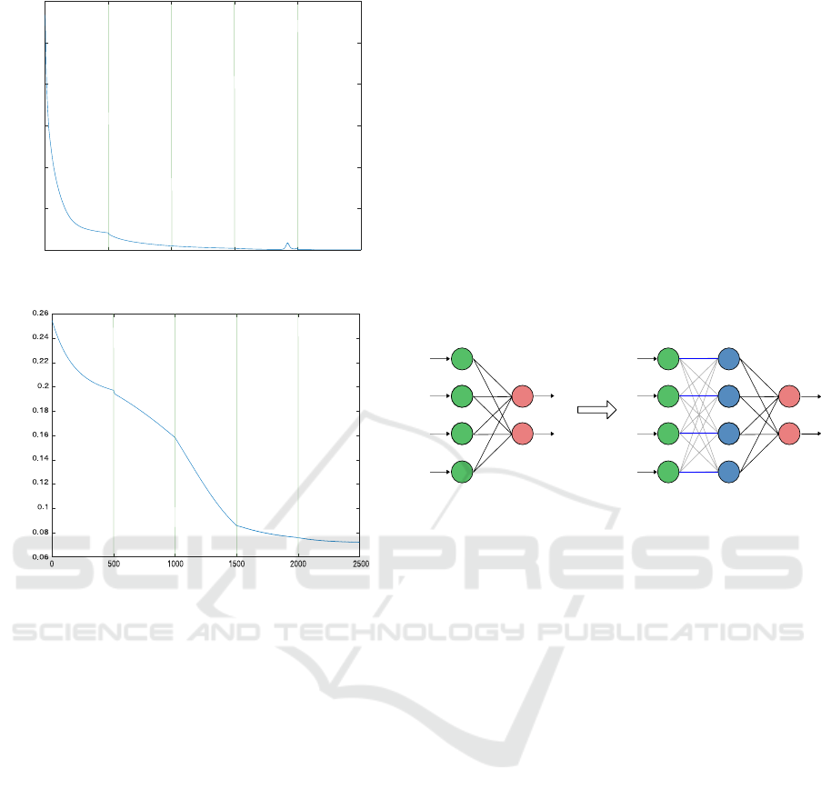
With this conﬁguration above, CollabNet obtained

a decay of the Mean Square Error (MSE) more efﬁ-

ciently, with the decay of the permanent error, when

compared to the MLP training without the method

proposed by this work, as shown in Figure 1. The

hit rate for this setup was 95.7%.

3.2 Method

This approach assumes that each new layer must be-

gin its training precisely from the point at which the

immediately preceding layer has stopped. In other

words, it is sought to decrease the error gradually,

even when another layer is inserted into the neural

network, as shown in Figure 2. Thus, this scheme

can provide increasing learning, avoiding traps of lo-

cal minimums or plateaus.

ICAART 2019 - 11th International Conference on Agents and Artiﬁcial Intelligence

686

MSE

Epoch

0 500 1000 1500 2000 2500

Figure 1: Decay of the MSE.

Epoch

MSE

Figure 2: Expected error behavior.

However, to succeed in this task, the integration

of the new layer must be properly performed, other-

wise the further layer may negatively affect the learn-

ing already achieved, causing a worsening in learning.

Therefore, the main idea of this proposal is to develop

a technique to incorporate the learning of the previous

layers in the training of the new layer, in order to pro-

vide knowledge about the learning already obtained

to a new layer.

The CollabNet structure is given according to

equation f (x) = w · f

(3)

(w · f

(2)

(w · f

(1)

(x))). In this

case, w represents the training weights of the layers,

(1)

is the activation function of the neurons of the

ﬁrst layer, f

(2)

of the second one and f

(3)

represents

the function of the third layer. The last layer is called

the output layer, and the network depth is given by the

total length of the layered chain.

3.2.1 Training

The training strategy proposed in this work starts

analogously to the traditional method of an MLP net-

work, with only one hidden layer and the use of

the backpropagation algorithm (Glorot and Bengio,

2010). After this ﬁrst stage of training, when the net-

work exit error does not decrease further, then a new

layer can be inserted into the training network. This

inclusion must necessarily be done one by one, since

after the insertion of a new layer it is necessary to

carry out several procedures, commented below, aim-

ing at the harmonious inclusion of the new hidden lay-

ers.

The proposed approach presents an innovative

way of inserting new layers. This method is intended

to ensure that new layers do not corrupt the network

exit error. For this, it is necessary that the output of

each neuron of the newly inserted layer is the same

value of the output of the corresponding neuron of the

previous layer considering all the input data (Figure

3).

Output Layer

Layer A Layer B

Output layer

Layer A

Figure 3: Insertion of a new layer.

In this proposal, the initialization of weights be-

tween layers A and B is performed randomly. This

initialization disturbs the network output error after

the inclusion of a new layer. Therefore, in order to

provide output of layer B equal to output of layer A,

that is, the output error is not disturbed at the insertion

of a new layer, it is necessary to provide treatment at

the output of the layer A. Otherwise there is no guar-

antee that the output of layer B is the same of layer

A, since the output of layer B will be altered by the

newly initialized weights and by the activation func-

tion of layer B neurons.

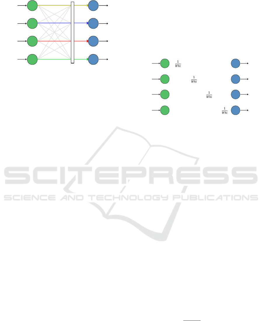
This work proposes to perform the data treatment

between layers A and B to compensate for the change

given by the newly created weights. This treatment

consists of a kind of mask, here called D, as shown

in Figure 4. The mask D modiﬁes the values that ar-

rive in the neurons of layer B, allowing that the output

of each neuron is exactly equal to the output of the

corresponding neuron in layer A.

The D mask ensures that each neuron in the new

layer receives only the inﬂuence of its corresponding

neuron from the previous layer. The operation of the

mask D is shown in Figure 4 and occurs as follows:

the connections represented by a colored line indicate

that the mask does not change the value, that is, the

neurons of the new layer B) receive exactly the output

value of the corresponding neuron in the anterior layer

(A). The connections represented by a gray line have

CollabNet - Collaborative Deep Learning Network

687

Layer A

Layer B

Figure 4: Mask D between an old layer and the newly in-

serted layer.

their value overridden by the mask, so the value re-

ceived from the adjacent neurons is null. In this way,

the input value of each neuron of the new layer is the

same value that leaves the neuron in layer A.

For the mask D to perform the ﬁlter as mentioned

earlier, there must be multiplication by the inverse of

the corresponding weight value, such that the value

effectively processed by the layer B neuron is exactly

the output value of the corresponding neuron of the

layer A. In this way, it is guaranteed that the training

of layer B will start exactly from the point where the

previous layer stopped. It is also ensured that new

insertions do not hinder the learning of the network

as a whole.

After the inclusion of layer B, it is then taken to

calculate the input of this layer, given by equation 1,

where W

i are the weights between layers A and B,

D is the mask and Y is the output of layer A. The .∗

operator means an element-by-element multiplication

and not a standard matrix multiplication.

net

= (W

. ∗ D) ∗Y (1)

In addition to the mask D, another modiﬁcation

proposed in this work consists in altering the activa-

tion function of the B layer neurons to, instead of sig-

moid, to be the identity function. In this way, what

enters the neurons of layer B becomes the output of

this layer. Thus, one has the guarantee that the output

of each neuron from layer B is exactly the output of

the corresponding neuron in layer A.

However, the innovations proposed in this work,

as they are, do not allow the new layer to acquire an

apprenticeship since the output of layer B will always

equal the output of layer A; therefore, there is no re-

duction of the network output error by modiﬁcation

of the new weights created. Thus, after insertion of

layer B, when the network training algorithm is ex-

ecuted, both the mask D and the activation function

of the neurons of layer B must change, to allow an

inﬂuence on the output from the Web.

However, abrupt withdrawal of the D mask and/or

the swapping of the sigmoid identity-activation func-

tion promote, on the one hand, the possibility of learn-

ing acquisition by layer B, but on the other hand, pro-

vide a sudden rise in error network. Thus, it is nec-

essary that there is a smooth and gradual transition

of mask removal D and the conversion of the identity

function to sigmoid.

ΔD

ΔD ΔD

ΔD

Layer A

Layer B

Figure 5: Change mask values D through ∆D.

The transition expressed in the previous paragraph

must occur during the execution of the training. Thus,

after a certain number of iterations (in this work it

was around 300), the weights between layers A and

B should promote the reduction of the output error

of the network, without prejudice to the decay of the

error promoted by the previous layers. This transfor-

mation is performed through a ∆D ranging from 0to1,

with speed deﬁned via parameterization of the initial-

ization of the new layer, as shown in Figure 5. In

this way, it is intended to ensure that the disturbance

caused by the insertion of a new layer hidden in the

network is the smallest possible.

While all the elements of the mask D varied uni-

formly, the elements of its main diagonal would vary

according to the random weights generated at the ini-

tialization of the new layer depending on the initial

values of those weights, the values of the main diago-

nal converge faster to one.

For this approach a sigmoid activation function

was used; however, its use is only performed when

the network is only a hidden layer. Thus, from the in-

clusion of the second hidden layer, it was necessary to

make a small adaptation in the sigmoid function, with

the intention of precisely controlling the inﬂuence of

the new layer in learning the network. This adaptation

is presented in Eq. 2.

(n) =

1 + e

−n

∗ c + n ∗ (1 − c) (2)

where φ

(n) is the output of the neuron with the

sigmoide

, c is the weighting factor of the activation

function and n is the weighted sum of all the synaptic

inputs of the neurons.

ICAART 2019 - 11th International Conference on Agents and Artiﬁcial Intelligence

688

The adaptation performed in Eq. 2 was imple-

mented by the need for the activation function to be

the identity function at the beginning of training of

a new layer. Throughout the training of this layer,

the activation function must be gradually converted

into the sigmoid function, which is promoted by the

c variable, so that after a certain amount of iterations,

the activation function returns to be only the sigmoid

function traditional. Thus, the variable c acts by

weighting the identity and sigmoid functions, trans-

forming an activation function of identity at the be-

ginning of the training of the new layer, to a sigmoid

function at the end.

The inclusion of the c variable in the sigmoid ac-

tivation function (φ) gives the designer the power to

control the inﬂuence of a layer in learning, in which

the closer to 1 is the value of the variable c, the greater

its inﬂuence and the closer to 0, the less will be such

inﬂuence. The use of the variable c in training is

of great importance for the method of inclusion of

new layers, because, with this artiﬁce, it is possible to

guarantee that the inﬂuence of the new layer is grad-

ual, as the weights of the new layer adjust to the prob-

lem, since, by default, these are generated randomly

for each new layer inserted.

Due to the change in the sigmoid activation func-

tion mentioned above, it was necessary to use the

derivative of the altered function in the backpropaga-

tion algorithm (Eq. 3).

dφ

= c · (y) · (1 − y) + (1 − c) (3)

where y is a traditional sigmoid function and c is the

weighting factor.

Using the D mask and the activation function

changed with the use of the variable c, the insertion of

a new layer did not interfere negatively in the learn-

ing, as it can be seen in the following chapter with

the presentation of the results obtained in the experi-

ments.

4 RESULTS AND DISCUSSION

CollabNet application was performed in a pattern

recognition task. The base used was the Wisconsin

Breast Cancer Dataset, withdrawn from the Machine

Learning Repository of the University of California

at Irvine (UCI). This database has information on 669

breast tumor registries, having two classes identiﬁed

as malignant (M) and benign (B) tumors, each with

ten calculated real characteristics for each cell nu-

cleus: radius, texture, perimeter, area, softness (local

variation in radius length), compactness (

perimetro

area−1.0

concavity (concave portions of the contour), concave

points, symmetry, and fractal dimension.

For this database, several conﬁgurations of the

proposed network were tested, varying several initial-

ization parameters, for both network and new layers:

number of neurons and epochs, learning rate, value

and moment of increment of variable c e of the mask

D (∆D) and the behavior of the weights in the train-

ing. However, the amount of neurons in the hidden

layers is a primary parameter that relates to the struc-

ture of the network. This parameter is deﬁned at the

moment of creation of the network, being immutable

from the insertion of the second hidden layer, ensur-

ing that each new layer hidden changes only the depth

of the network and not its width.

4.1 Parameterization

The training parameters were estimated empirically

and always with the inclusion of a new layer. The

learning rate, the number of times, the behavior of

the weights of the new layer in relation to its initial-

ization are essential parameters of the insertion of a

new layer. Finally, we have the parameters related to

the behavior of the variable c and the mask D, deﬁn-

ing information regarding the velocities of variation

of these variables in training.

Given the various parameters of the network, the

variable c deserves a more comprehensive explana-

tion, which in this project plays a special role. This

variable is directly related to the inclusion of a new

layer, as well as its transition, so that a newly in-

serted layer, not useful for learning the network, can

become an element of importance to this learning, as

presented in the Section 3. The variable c has the

responsibility to control the inﬂuence of a new layer

in training, being that inﬂuence is a quantity directly

proportional to the value of c, that is, the closer the

c is of its value (1), the higher the inﬂuence of the

new layer in training. Therefore, the control of c is

the great challenge of this proposal and the way that

the value of this variable increases during the training

of the new layer needs to be parameterized individu-

ally. The parameterization occurred empirically, with

values between 0.001 and 0.003 being chosen.

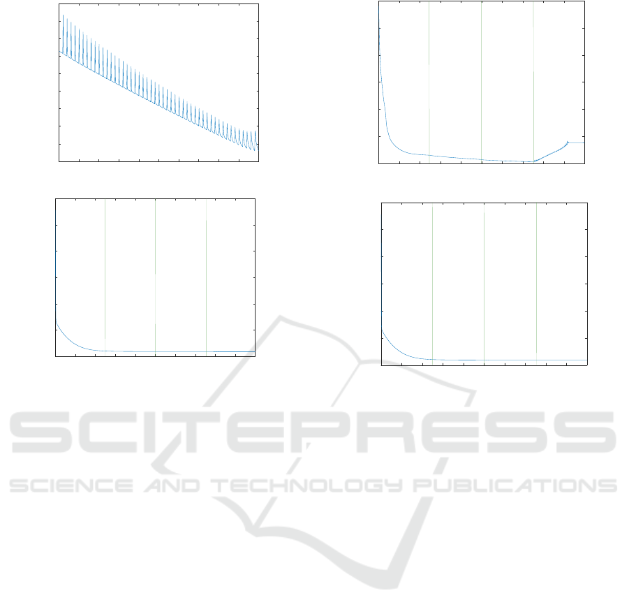
The designer must carefully observe the adjust-

ment of the increment of c since its correct parame-

terization has a direct inﬂuence on the behavior of the

MSE. Figure 6(a) presents an enlarged view of the last

training layer shown in Figure 6(b), wherein this in-

clusion an increment of the variable c relatively high

was deﬁned, approximately 0.3 at each iteration. In

each iteration of c, it is possible to perceive the pertur-

bations in the MSE. This phenomenon is explained by

CollabNet - Collaborative Deep Learning Network

689

MSE

Epoch

0 50 100 150 200 250 300 350 400 450 500

0.0366

0.0367

0.0368

0.0369

0.037

0.0371

0.0372

0.0373

0.0374

0.0375

(a) Variable c with high incremental value

MSE

Epoch

0 200 400 600 800 1000 1200 1400 1600 1800 2000

2.5

1.5

0.5

(b) Variable c with low incremental value

Figure 6: The behavior of MSE variations of c.

a high variation of the variable c and by the weights

that are not yet close to the convergence of the ﬁnal

value.

In Figure 6(b), the MSE is presented shortly after

the inclusion of a new layer with an increment of the

variable c relatively low. In this case, the inﬂuence of

the new layer is low and this new layer increases the

training time.

Also the variable c, the mask variation D also

plays a vital role in the inclusion and control of new

layers, necessitating that it be observed in the act of

inserting new layers, considering that ∆D has its vari-

ation intrinsic to the incremental value of c and is di-

rectly related to the mask transformation D. The cor-

rect parameterization of ∆D is essential for training

since this parameter together with the variable c con-

trols the inﬂuence of the new layer in the global train-

ing. The mask D must be started with 0, the exception

of the main diagonal and its update is carried out si-

multaneously with the variable c by the value ∆D.

A non-harmonious conﬁguration of these param-

eters results in the undesirable behavior of the MSE,

and consequently impairs training. As an example of

such undesirable behavior, cases are shown wherein

∆D is high 1 and low 2, respectively. This parame-

ter refers to the speed that mask D is invisible to the

training, that is, the process of inclusion of the new

layer has been completed.

MSE

Epoch

2.5

1.5

0.5

0 200 400 600 800 1000 1200 1400 1600 1800 2000

(a) ∆D with high value

MSE

Epoch

0 200 400 600 800 1000 1200 1400 1600 1800 2000

2.5

1.5

0.5

(b) ∆D with low value

Figure 7: The behavior of MSE variations of ∆D.

Figure 7(a) shows an undesired behavior in the

last layer, caused by the convergence velocity of the

mask D. In Figure 7(b), another unwanted behavior

is presented, where the inﬂuence of the new layer is

practically null because the updating rate of ∆D was

relatively small.

Another major challenge in CollabNet’s parame-

terization, as in any MLP-based approach, is the deﬁ-

nition of the learning rate. This parameter is directly

related to the learning speed of the network. At Col-

labNet, the learning rate may be different for each

layer. In this way, it is necessary that the designer

has the sensitivity and the ability to deﬁne the value

of the learning rate for each layer. Figure 8(b) illus-

trates the CollabNet output, with three hidden layers

and the relatively low learning rate value (5x10

−5

In this example, the output MSE behavior is dis-

played with a low learning rate. Thus, the MSE tends

to continue the output of the network in previous lay-

ers, without promoting any improvement in the decay

of the output error.

In Figure 8(a), the error behavior is presented with

the inclusion of a new layer, now with learning rate

having a relatively high value (0.1). It is possible to

observe that the tendency of the error, in this case,

is to initially lower and soon after increasing sharply

with each increment of c. This behavior is explained

ICAART 2019 - 11th International Conference on Agents and Artiﬁcial Intelligence

690

MSE

Epoch

(a) MSE with high learning rate value

MSE

Epoch

(b) MSE with low learning rate value

Figure 8: MSE for variations of learning rate.

by the fact that with the high learning rate at a time

where the weights of the new layer still do not con-

form to the weights already trained in previous lay-

ers, thus generating a greater disturbance in the MSE.

This fact can be still perceived, observing in the ﬁnal

graphics part, where the weights are already more ad-

equate for the rest of the training, so the perturbation

of the NDE with each new increment of c is smaller.

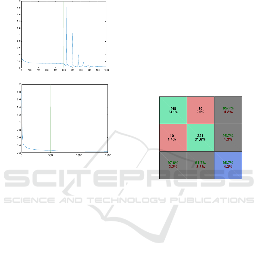
4.2 Validation Metrics

In this work, the confusion matrix and receiver op-

erating characteristic (ROC) were used as evaluation

metrics. With the confusion matrix, one can check the

network performance in the task of sorting patterns,

regardless of the class. Figure 9 presents the confu-

sion matrix obtained from the experiment quoted in

this section, ﬁnalized with ﬁve hidden layers. In this

ﬁgure, class 1 represents benign cases, and class 2

represents malignant cases, the ﬁrst two diagonal cells

show the number and percentage of correct classiﬁ-

cations by CollabNet, that is, 448 biopsies were cor-

rectly classiﬁed as benign (True Negative - TN) and

221 cases were correctly classiﬁed as malignant (True

Positive - TP), corresponding respectively to 64.1%

and 31.6% of the 699 biopsies. 20 samples (2.9% of

total) of the malignant biopsies were incorrectly clas-

siﬁed as benign (False Positive - FP). Similarly, ten

biopsies (1.7 % of the data) were improperly classi-

ﬁed as malignant (False Negative - FN).

Of the 468 benign predictions, 95.7% were cor-

rect and 4.3%, erroneous. Of the 231 malignant pre-

dictions, coincidentally, 95.7% were accurate and 4.3

%, incorrect. Of the 458 benign cases, 97.8% of the

cases were correctly predicted to be benign, and 2.2%

were predicted to be malignant. Of the 241 malignant

cases, 91.7% were correctly classiﬁed as malignant

and 8.3% as benign.

Overall, 95.7% of predictions were correct, and

4.3% were wrong classiﬁcations.

Output classes

Target classes

TN FN

TPFP

Figure 9: Matrix of confusion at the end of training.

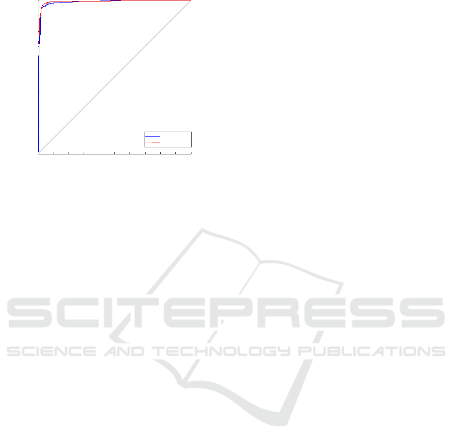
Another metric used in the evaluation of Collab-

Net is the ROC, or ROC curve, where for each class of

this classiﬁer, there are values in the interval of [0,1]

for each output. For each class, two values are cal-

culated, the TP Rate or sensitivity and the FP Rate

or speciﬁcity. Therefore, sensitivity is the ability of

the system to correctly predict the condition for cases

that have it, whereas uniqueness is the ability of the

system to predict cases that do not have a certain con-

dition precisely.

Figure 10 illustrates the ROC plot for the Collab-

Net conﬁguration presented in this section, where the

closer to the top left is the graph lines, the better the

ranking.

In this graph it is possible to see that both classes,

malignant (blue) and benign (red) tumors, have their

curves near the upper left corner, demonstrating the

efﬁciency of the method in the classiﬁcation of the

selected database. However, a greater approxima-

tion of the curves at the point of interest of the ROC

curve must be object of constant search in any ma-

chine learning algorithm. In this way, parameter ad-

justments and more validation tests are essential in the

search for better classiﬁer results.

CollabNet - Collaborative Deep Learning Network

691

Benign

Malignant

0 0.1 0.2 0.3 0.4 0.5 0.6 0.7 0.8 0.9 1

0.9

0.8

0.7

0.6

0.5

0.4

0.3

0.2

0.1

Figure 10: ROC plot.

5 CONCLUSIONS

This work proposes a training architecture inspired by

layered stacking techniques; however, this approach

goes hand in hand with the classic stacking since there

is no need to corrupt data entry for each new layer. In

this way, greater training control is achieved, start-

ing the training of a new layer always from the point

where the network stopped. For that, a change was

performed in sigmoid function allowing to control the

inﬂuence of the new layer in the global training of the

network.

The results obtained in the experiments of this

work demonstrate that this approach has a promis-

ing future regarding a new RNA concept, where good

results were obtained even with some training disci-

plines. The way how to process variable c and the use

of an intelligent algorithm to identify the ideal time

for the inclusion of a new layer are possible outcomes

of this work.

ACKNOWLEDGMENTS

The authors would like to acknowledge technical

and ﬁnancial supports from the UFMA, FAPEMA,

MecaNET, IFTO and UNICEUMA.

REFERENCES

Arjovsky, M., Chintala, S., and Bottou, L. (2017). Wasser-

stein Generative Adversarial Networks. Proceedings

of The 34th International Conference on Machine

Learning, 70:214–223.

Bengio, Y. (2009). Learning Deep Architectures for

AI. Foundations and Trends

 in Machine Learning,

2(1):1–127.

Bengio, Y., Lamblin, P., Popovici, D., and Larochelle, H.

(2006). Greedy Layer-Wise Training of Deep Net-

works. Advances in Neural Information Processing

Systems 19 (NIPS’06).

Glorot, X. and Bengio, Y. (2010). Understanding the difﬁ-

culty of training deep feedforward neural networks. In

Teh, Y. W. and Titterington, M., editors, Proceedings

of the Thirteenth International Conference on Artiﬁ-

cial Intelligence and Statistics, volume 9 of Proceed-

ings of Machine Learning Research, pages 249–256,

Chia Laguna Resort, Sardinia, Italy. PMLR.

Goodfellow, I., Pouget-Abadie, J., Mirza, M., Xu, B.,

Warde-Farley, D., Ozair, S., Courville, A., and Ben-

gio, Y. (2014). Generative Adversarial Nets. In Ad-

vances in Neural Information Processing Systems 27,

pages 2672–2680.

Huang, X., Li, Y., Poursaeed, O., Hopcroft, J., and Be-

longie, S. (2016). Stacked Generative Adversarial

Networks. Iclr, pages 1–25.

Larochelle, H., Erhan, D., and Vincent, P. (2009). Deep

Learning using Robust Interdependent Codes. Pro-

ceedings of the Twelfth International Conference on

Artiﬁcial Intelligence and Statistics (AISTATS 2009),

5:312–319.

Lecun, Y., Bengio, Y., and Hinton, G. (2015). Deep learn-

ing. Nature, 521(7553):436–444.

Netanyahu, N. S. (2016). Deeppainter : Painter classiﬁ-

cation using deep convolutional autoencoders. In In-

ternational Conference on Arti cial Neural Networks

(ICANN), volume 9887, pages 1–8.

Schmidhuber, J. (2014). Deep learning in neural networks:

An overview. Neural Networks, 61:85–117.

Vincent, P. and Larochelle, H. (2010). Stacked denois-

ing autoencoders: Learning useful representations in

a deep network with a local denoising criterion pierre-

antoine manzagol. Journal of Machine Learning Re-

search, 11:3371–3408.

Wolberg, W. H., Street, W. N., and Mangasarian, O. L.

(2011). UCI Machine Learning Repository: Breast

Cancer Wisconsin (Diagnostic) Data Set.

ICAART 2019 - 11th International Conference on Agents and Artiﬁcial Intelligence

692