Analytic Surface Detection in CAD Exported Models

Pavel

Sigut

, Petr Van

cek

and Libor V

Department of Computer Science and Engineering, University of West Bohemia, Technick

a 8, Plze

n, Czech Republic

NTIS - New Technologies for the Information Society, University of West Bohemia, Technick

a 8, Plze

n, Czech Republic

Keywords:

Analytic Surface, Fitting, Curvature, Estimation, Analysis, CAD.

Abstract:

3D models exported from CAD systems have certain speciﬁcs, that inﬂuence their subsequent processing.

Typically, in contrast with scanned surface meshes, vertices of exported meshes lie almost exactly on analytic

surfaces used in CAD modeling. On the other hand, the triangulation of exported models is usually dictated by

the requirement of having the lowest possible number of primitives, which results in highly uneven sampling

density and common appearance of extremely large and small triangle inner angles. For applications such as

classiﬁcation, categorization, automatic labeling or similarity based retrieval, it is often necessary to identify

signiﬁcant features of an exported model, such as planar, cylindrical, spherical or conical regions, and their

properties. While this type of information is naturally available in the original CAD system, it is only rarely

exported together with the surface model. In this paper, we discuss two means of identifying analytic regions

in triangle meshes, taking into account the speciﬁcs of CAD-exported models, and provide a quantitative

comparison of their performance.

1 INTRODUCTION

In certain applications, large sets of 3D models are

exported from a CAD system in the form of triangle

meshes and further processed in this format. Com-

monly, a very basic ﬁle format, such as .STL, is in-

tentionally chosen in order to maximize compatibil-

ity. Apart from being rather inefﬁcient at represent-

ing the mesh connectivity, such format does not in-

clude any additional information about the original

CAD part. The subsequent processing, which might

include classiﬁcation, categorization, automatic label-

ing or similarity based retrieval, can greatly beneﬁt

from availability of information such as number, lo-

cations and radii of cylindrical holes in the model and

similar high level properties. However, such infor-

mation is lost during the export, and for reasons of

compatibility with multiple CAD tools, it is generally

not an option to deﬁne a custom export format that

includes such data.

In particular, common CAD models, such as tech-

nical workpieces or models of buildings, generally

consist of patches deﬁned by simple geometric primi-

tives, such as planes, cylinders, spheres, cones, less

often also tori and more general surfaces. These

patches are tessellated during the export, and thus

turned into piecewise planar surfaces. Our speciﬁc

objective is to identify these patches, together with

Figure 1: Example of a typical model exported from a CAD

system. Notice the extremely small inner angles.

the parameters of the original geometric primitives.

For each resulting primitive, a set of triangles is to be

found that represent it in the model. For CAD mod-

els, it is reasonable to expect that the vertices of the

triangles assigned to a particular patch lie almost im-

mediately on a surface deﬁned by the primitive, only

allowing for a numerical imprecision.

A similar problem has been addressed by many

works concerning analysis, completion and reﬁne-

ment of scanned triangle meshes. We argue that al-

though these problems are related, there are circum-

stances that make them substantially different. In par-

ticular, scanned 3D meshes usually have a relatively

uniform sampling that is dictated by the resolution of

278

Šigut, P., Van

cek, P. and Váša, L.

Analytic Surface Detection in CAD Exported Models.

DOI: 10.5220/0007396702780285

In Proceedings of the 14th International Joint Conference on Computer Vision, Imaging and Computer Graphics Theory and Applications (VISIGRAPP 2019), pages 278-285

ISBN: 978-989-758-354-4

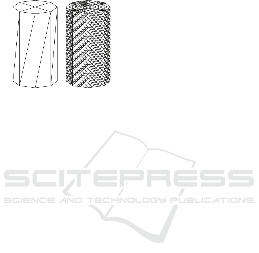
Figure 2: Cylinders are often represented by a low number

of sides (left). However, subdividing them in order to im-

prove triangle regularity is not possible, because the result-

ing shape (right) is rather interpreted as a ﬂat sided prism

than a cylinder.

the sampling device. A CAD exported model, on the

other hand, usually has a tessellation that is minimal

with respect to the original shape. Therefore there are

many elongated triangles, and even important parts

are often represented by only a very few triangles.

Resampling a CAD exported model regularly, al-

though possible, is generally not a viable approach. A

CAD-exported model usually has all vertices exactly

(up to numerical error) lying on the analytic surfaces

used in the design process. Any resampling always

introduces additional vertices, whose position cannot

be determined so that they also lie on the actual sur-

face of the model (for illustration see Figure 2). On

the other hand, the vertex positions in scanned data

always contain noise that must be taken into account,

which is an issue that rarely occurs with CAD exports.

We have experimented with two fundamentally

different approaches to the problem at hand. First

is based on estimating principal curvatures for each

mesh vertex, which in turn allows us to classify ver-

tices as either planar, cylindrical and possibly spher-

ical. Next, continuous patches of vertices that lie on

a common plane, cylinder or sphere are created using

a region growing technique. Finally, the equation of

each segment is reﬁned.

The curvature based approach depends strongly

on the quality of curvature estimation, which is in

turn dictated by the sampling quality that is typically

rather poor with CAD exported models. Therefore

we have experimented with another, more direct ap-

proach to the problem at hand. Basic primitives, such

as planes, cylinders, spheres and cones are ﬁtted to

local patches of triangles. If a good ﬁt is found, the

segment is then grown by traversing the surface. The

parameters of the representing primitives are reﬁned

using a gradient descent based approach.

After reviewing related work in the following sec-

tion, sections 3.1 and 3.2 will discuss both approaches

in more detail. Note that although some of the de-

sign choices in the algorithm description may seem

arbitrary, we have performed extensive testing of a

plethora of variations, trying to achieve best possible

results in experiments that will be described in section

4. The algorithm ﬂow and parameters described here

result from these experiments and provide the best re-

sults we were able to achieve by either method. Fi-

nally, section 5 will compare the two approaches and

section 6 will conclude the paper.

2 RELATED WORK

Previous work mostly addresses the problem of ﬁnd-

ing analytic surfaces in dense scanned meshes, mostly

in the context of reverse engineering (V

arady et al.,

1997)(Benk

o et al., 2001)(Benk

o et al., 2002). A

bottom-up approach ﬁtting planes, spheres and cylin-

ders has been proposed by (Attene et al., 2006). Prim-

itives are ﬁtted to small patches ﬁrst, and the patches

are merged in a greedy fashion in order to obtain

larger consistent areas.

An approach based on sampling the surface ran-

domly and searching for ﬁtting planes, cylinders,

cones, spheres and tori has been proposed by (Schn-

abel et al., 2007). This approach has been later used

for ﬁlling in missing parts of scanned man made ob-

jects (Schnabel et al., 2009).

Another approach based on extracting and opti-

mizing boundary curves on the primitive shapes has

been proposed by (Jenke et al., 2008). The method is

primarily targeted at scanned indoor/outdoor scenes

with noise and outliers.

Fitted surfaces were also used by (Li et al., 2011)

in order to discover global relations, such as symme-

tries and parallel planes. This kind of global relations

help adjusting the parameters of the ﬁtted surfaces and

improve the reconstruction quality.

Identifying local proxies, i.e. planar or other an-

alytical surfaces, is also a key ingredient in Vari-

ational Shape Approximation(VSA) (Cohen-Steiner

et al., 2004) and its more advanced variants (Wu and

Kobbelt, 2005). While the original VSA algorithm

only uses planes as proxies, the Hybrid Variational

Surface Approximation also allows using spheres and

cylinders as well.

The primitive ﬁtting based approach we describe

is closely related to algorithms discussed in the litera-

ture. On the other hand, using curvatures for identify-

ing analytic patches in triangle meshes has to the best

Analytic Surface Detection in CAD Exported Models

279

of our knowledge not been thoroughly studied before.

3 ALGORITHMS

3.1 Curvature based Detection

The curvature based detection algorithm consists of

following steps:

1. Preprocessing. Mesh is cut along crease edges

and extremely long triangles are subdivided into

smaller ones.

2. Curvature Estimation. Principal curvatures are

estimated for each vertex of the preprocessed

mesh.

3. Vertex Classiﬁcation. Each vertex is marked as

either planar, cylindrical or other based on the cur-

vatures.

4. Patch Creation. Continuous patches of vertices

of the same type are identiﬁed.

5. Primitive Fitting. Parameters of the correspond-

ing primitives are estimated for each patch.

6. Vertex-triangle Mapping. The primitives repre-

sented as vertex sets are transformed into sets of

triangles of the input mesh (i.e. before subdivi-

sion).

7. Postprocessing. Large primitives with a good ﬁt

are grown to include possible neighbouring trian-

gles that also ﬁt their equation. Small patches are

removed.

Each of these steps will be discussed in the following

paragraphs in more detail.

3.1.1 Preprocessing

First, any non-manifold edges and vertices of the

mesh are removed. Next, the continuous mesh is split

along edges where the dihedral angle is larger than

◦

. This threshold is chosen experimentally, based

on the knowledge that regular 8-sided prisms (45

◦

di-

hedral angles) commonly appear in CAD models, and

their sides therefore should be separated, while higher

side count usually indicates the presence of a cylinder,

where the mantle should remain continuous.

As a second step, elongated triangles are subdi-

vided. A threshold is determined based on the me-

dian edge length, and on each edge longer than the

threshold new vertices are generated. Finally, all tri-

angles incident with subdivided edges are split into

smaller triangles ﬁlling the area of the original trian-

gle. This step is necessary for the following curva-

ture estimation to succeed, however, as argued previ-

ously, global remeshing of the surface is not a viable

option. In the experiments we have performed, the

above described process provided better results than

both working with original geometry and full resam-

pling.

3.1.2 Curvature Estimation

Many approaches to estimating curvature on sampled

surface have been proposed in the literature (for a re-

cent review, see (V

sa et al., 2016)). We have tested

multiple choices, obtaining best results using the gen-

eralized shape operator approach by Hildebrandt et al.

(Hildebrandt and Polthier, 2011). In particular, we

have used the

S operator with radius equal to 1.6 × a,

where a is the average edge length in the triangle

mesh. This method allows us to estimate both prin-

cipal curvatures at each mesh vertex with reasonable

accuracy and robustness.

3.1.3 Vertex Classiﬁcation

Next, each vertex is classiﬁed as either planar, cylin-

drical or unknown. A vertex is classiﬁed as planar,

when both its curvatures are smaller than 5% of the

average curvature over all vertices. Otherwise, a ver-

tex may be classiﬁed as cylindrical, if the ratio of the

magnitudes of the estimated principal curvatures is

larger than 10:1. Finally, if this condition is not met

either, the vertex is classiﬁed as unknown. Note that

it would be fairly easy to classify vertices as spheri-

cal by principal curvature equality, however, we did

not use this classiﬁcation, since spherical segments

are rather rare in the data we have experimented with.

In contrast with that, detecting a conic vertex is gen-

erally not possible by looking only at a single vertex

and its estimated principal curvatures.

3.1.4 Patch Creation

Having a vertex classiﬁcation, continuous surface

patches are generated in the next step. From each ver-

tex that is not classiﬁed as unknown, a breadth ﬁrst

search is started using the mesh connectivity. Ver-

tices are added to the patch if they are of the same

type, and their estimated curvature is not too different

from that of the initial vertex. In order to evaluate the

similarity, we relate the difference in curvature to the

average curvature over all vertices of the mesh. If the

magnitude of the difference is larger than 10% of the

average curvature in either of the principal curvatures,

then the candidate vertex is deemed too different and

GRAPP 2019 - 14th International Conference on Computer Graphics Theory and Applications

280

is not added to the growing patch. Otherwise, it is

conquered and marked as such, so that it is neither

later used in any other patch nor as initial vertex for

another search.

3.1.5 Primitive Fitting

For each patch, a corresponding primitive is ﬁtted.

Plane ﬁtting is done in the least squares sense. Cylin-

ders, on the other hand, are ﬁtted by a two stage pro-

cess. First, a unit direction is found that has the small-

est dot product with all vertex normals in the patch,

by solving an eigenvalue problem resulting from the

constrained minimization. This direction is the likely

orientation of the axis of the cylinder. Next, all ver-

tices are projected along this direction, forming a set

of 2D points, which are ﬁtted by a circle. We start

with a set of equations in the form

− x

)

+ (y

− y

)

= r

, (1)

where x

, y

are the projected coordinates of i-th

point, x

, y

are the unknown coordinates of the center

and r is the unknown circle radius. Expanding the

equation yields

− 2x

+ x

+ y

− 2y

+ y

= r

. (2)

Subtracting an arbitrary j-th equation from all oth-

ers results in a set of linear equations of form

− 2x

+ y

− 2y

− x

+ 2x

− y

+ 2y

= 0,

(3)

which is solved in the least squares sense. The re-

sulting center point corresponds to the cylinder axis,

and the cylinder radius is computed as the average dis-

tance of all vertices in the segment to this axis.

3.1.6 Vertex-triangle Mapping

So far, patches of vertices are identiﬁed, our goal is,

however, to obtain triangle patches. In the mapping

step, a conversion is performed. If a vertex is assigned

to a patch, all of its incident triangles are marked as

claimed by the given patch. These triangles may be

the result of triangle splitting performed in prepro-

cessing, for each such triangle we keep the index of

the original triangle it comes from, and this triangle

is then claimed by the patch. This way, each origi-

nal triangle may be claimed three times by the same

patch, or possibly by several different patches differ-

ent number of times. Conﬂicts are resolved based on

the number of claims: the patch that claims a triangle

most times gets it assigned. This way, some minor

patches disappear completely.

3.1.7 Postprocessing

Since some vertices may ﬁt into multiple patches,

some triangles may be assigned to a wrong patch at

this point, especially those on the border between

patches. As a ﬁnal step, patches are sorted in order of

descending area, and grown. For each patch, neigh-

bouring triangles are considered, and the tip vertex

of each neighbouring triangle is tested for ﬁt to the

given patch. If it is close enough to the analytic sur-

face represented by the patch, it is reassigned, unless

it is already assigned to a larger patch. If a triangle

is reassigned to a patch, its neighbours are considered

for reassignment as well.

3.2 Gradient Descent

The above described method suffers from issues re-

lated to the key component of vertex curvature esti-

mation. Therefore we have implemented a different

approach as well, building on different concepts. In

particular, we use analytic expression for squared dis-

tance from each ﬁtted primitive. This allows us to ﬁt

primitives to vertex sets using a gradient descent ap-

proach. The algorithm works in following steps:

1. Plane Fitting. Parameters of a plane equation are

computed for each local neighbourhood and pla-

nar regions are grown using a traversal technique.

2. Cylinder Fitting. Parameters of a cylinder equa-

tion are estimated for each local neighbourhood

and reﬁned using gradient descent. Additional

triangles are added to the patch using a traversal

technique.

3. Cone Fitting. Parameters of a cone equation are

estimated for each local neighbourhood and re-

ﬁned using gradient descent. Additional triangles

are added to the patch using a traversal technique.

4. Judging. Triangles that are part of multiple

patches are assigned to a single patch using a de-

cision algorithm.

Note that this approach does not use triangle sub-

division as the curvature based algorithm did, since it

is not necessary. On the other hand, splitting edges

with large dihedral angle is still performed.

3.2.1 Plane Fitting

Each triangle of the triangle mesh deﬁnes a plane.

During plane ﬁtting, plane equation parameters are

computed for each triangle that is not yet assigned

to a plane patch. Next, using breadth ﬁrst search,

neighbouring triangles are tested whether or not they

ﬁt into the equation, and ﬁtting triangles are added to

Analytic Surface Detection in CAD Exported Models

281

the growing patch. Patches consisting of a single tri-

angle are discarded, all others are preserved for the

ﬁnal judging.

3.2.2 Cylinder Fitting

Next, a similar process is done for ﬁtting cylinders.

Tetriamonds, i.e. quadruples of neighbouring trian-

gles, are generated starting from triangles that are not

assigned to any cylinder patch yet. For each tetria-

mond, an initial cylinder is found using the same pro-

cedure as described in section 3.1.5, only this time us-

ing triangle normals and triangle centroids instead of

vertices and their normals to estimate cylinder orien-

tation, since the triangle normals are more represen-

tative of the surface. Next, we build an analytic equa-

tion for squared distance from the cylinder surface.

Partial derivatives of this equation are computed with

respect to all cylinder parameters. Using the deriva-

tives, gradient descent is used to optimize the param-

eters of the cylinder so that it ﬁts the vertices of the

tetriamond as closely as possible. If the ﬁnal ﬁt is

tight enough, the cylinder patch is preserved and ad-

ditional triangles are assigned to it using breadth ﬁrst

search.

3.2.3 Cone Fitting

Cones are ﬁtted in a way similar to cylinder ﬁtting.

Normals of points lying on a cone all lie on a plane

that is orthogonal to the orientation of the cylinder

(see Fig. 3). Once again, we use triangle normals and

triangle centroids of a tetriamond consisting of trian-

gles not yet assigned to any cone. Fitting a plane to

the normals in least squares sense allows us to esti-

mate the direction of a potential cone. Average angle

between the normals and the estimated cone direction

allows us to estimate the cone angle, and combined

with the cone direction it is possible to estimate the

cone apex position.

Next, we improve the cone equation in the same

way cylinder equation has been improved. Since dis-

tance to a cone is not as straightforward as distance

to a cylinder, we describe the used formula in more

detail. Squared distance d of a point x from a cone

with apex o, unit axis direction v and tip angle α (see

ﬁgure 4) can be expressed as

d(x, o, v, α) = sin

(β − α) ∗ (x − o) · (x − o), (4)

where

cosβ =

(x − o) · v

kx − ok

. (5)

Figure 3: A cone with a few random surface points and their

normals (left). When the normals are brought to a common

origin (right), they all lie in a plane (dashed) that is orthog-

onal to the cone axis direction (dotted).

Figure 4: Variables in the distance from cone computation.

For the purposes of efﬁcient computation, the ﬁrst

term in equation 4 can be written as

sin

(β − α) = (sinβcosα − cosβsinα)

, (6)

where cosβ can be obtained from equation 5 and

sinβ = (1 − cos

β)

. Note that this expression is cor-

rect for both points inside and outside of the cone.

Equation 4 can be differentiated with respect to all

cone parameters, which allows us to use gradient de-

scent in order to reduce the squared distances of ver-

tices from the cone. Cones that ﬁt tetriamond vertices

are grown again by a breadth ﬁrst search. In contrast

with cylinders, whenever we reach a vertex that does

not ﬁt the cone, we reﬁne the cone parameters using

the gradient descent procedure once more, taking into

account all previously added vertices. This is neces-

sary, since the cone ﬁtting is more prone to getting

trapped in a local minimum. Once the parameters are

reﬁned, the previously unﬁt vertex is tested again and

if it ﬁts, it is added to the patch and the search proce-

dure continues.

GRAPP 2019 - 14th International Conference on Computer Graphics Theory and Applications

282

Figure 5: A typical result of classiﬁcation. Different planes

are marked in different shades of red, cylinders in green,

cones in blue. Curvature is unable to ﬁnd the conic surface

and ﬁts several cylinders instead (left), while gradient cor-

rectly ﬁts a single cone (right).

3.2.4 Postprocessing

At this point, each triangle can be claimed by up to

three patches: a plane, a cylinder and a cone. A deci-

sion algorithm assigns each triangle to a single patch,

selecting the largest patch in terms of total number

of claimed triangles. After this step, each triangle

is assigned to a single patch. Finally, assignment is

reﬁned by the same procedure as described in sec-

tion 3.1.7, i.e. patches are processed from largest to

smallest and possible reassignments of neighboring

vertices are considered and performed.

4 EXPERIMENTS

In order to test the performance of the two described

methods (abbreviated as curvature and gradient), we

have designed an experiment that compares the re-

sults with manually tagged data. A person that was

otherwise not involved with the development of ei-

ther method was given a set of exported CAD models.

They were requested to select groups of triangles on

each model and mark them as plane, cylinder or cone.

On each model, multiple groups could be selected,

and each group should always contain triangles that

belong to a single analytic surface. They were not re-

quired to mark all the triangles of each model, and in

areas where the classiﬁcation was uncertain they were

speciﬁcally instructed not to perform marking.

In total, 95 models were marked, ranging from 12

to 80 000 triangles. In total, there were 81597 out of

225068 triangles marked in 1919 groups, out of which

1136 were plane groups, 636 were cylinder groups

and 147 were cone groups.

This data allows us to evaluate several accuracy

criteria. First, for each marked triangle, we can

check whether or not each method has assigned it to

Table 1: Percentages of incorrectly classiﬁed triangles. Av-

erage values are listed with corresponding standard devia-

tions in parentheses.

method cones on cones off

curvature 9.06% (15.22%) 3.44% (10.52%)

gradient 4.67% (12.90%) 2.85% (11.61%)

the correct primitive type. Second, for each group,

we can check whether all triangles belonging to the

group were also assigned to a single patch by each

method, and no classiﬁed patch falls into more than

one marked group.

Since the principle of the curvature based method

makes it unable to detect cones, although they appear

quite commonly in our data, we must decide how to

handle their evaluation and avoid bias towards either

method (see ﬁgure 5). There are two approaches pos-

sible, both of which we have tested:

1. for curvature, consider all triangles that were

marked as cone and classiﬁed as anything but un-

known as an error (denoted cones on).

2. turn off cone classiﬁcation in gradient and ignore

all triangles marked as cone (denoted cones off ).

5 RESULTS

Table 1 lists the percentages of incorrectly classiﬁed

triangles for both methods. It shows that both meth-

ods present a viable approach to the problem at hand.

The gradient based method provides slightly better re-

sults. The considerably large values of standard devi-

ation indicate that with most models most triangles

were classiﬁed correctly (in fact, median of all per-

centages in the table is 0.0%), while there are a few

problematic cases where large error percentages oc-

cur.

Most interestingly, the Pearson correlation co-

efﬁcient of the error percentages of the curva-

ture/gradient based methods is -0.025 for the cones on

scenario and -0.058 for the cones off scenario. This

indicates, that rather than some models being more

difﬁcult than others, it is more likely that different

models cause problems with either method (see ﬁg-

ure 6). A potential hybrid method that combines the

strengths of both discussed approaches could there-

fore achieve a considerable improvement of classiﬁ-

cation accuracy.

Sometimes, it might happen that a small area of a

model is densely sampled, and if it gets incorrectly

classiﬁed, then it may skew the overall results. In

table 2 we list the percentages of marked areas that

were classiﬁed incorrectly. Interestingly, in this crite-

Analytic Surface Detection in CAD Exported Models

283

10%

20%

30%

40%

50%

60%

70%

80%

90%

100%

0% 10% 20% 30% 40% 50%

percentage of incorrect triangles,

gradient, cones on

percentage of incorrect triangles, curvature, cones on

Figure 6: Correlation of the percentage of incorrectly clas-

siﬁed triangles by both methods.

Table 2: Percentages of incorrectly classiﬁed surface areas.

Average values are listed with corresponding standard devi-

ations in parentheses.

method cones on cones off

curvature 3.29% (9.60%) 1.66% (7.61%)

gradient 4.63% (15.63%) 4.01% (15.61%)

rion, the curvature based approach provides better re-

sults regardless of whether or not cone classiﬁcation

is considered.

Additionally, we can also evaluate the consistence

of whole marked groups rather than individual trian-

gles. For each marked group, we check two fail cases:

1. Triangles of the group are part of two or more

classiﬁed patches.

2. Another marked group contains triangles classi-

ﬁed to the same patch.

Note that the two cases are not equivalent: if a classi-

ﬁer puts all cylinder triangles into a single patch, then

the ﬁrst case does not occur, since for each marked

group, all of its triangles fall into a single classi-

ﬁed patch. If either of these cases occurs, we mark

the group as incorrectly identiﬁed. Table 3 lists the

percentages of incorrectly identiﬁed groups for both

tested methods in both tested scenarios. Curvature

provides here substantially better performance than

gradient in terms of both average values and standard

deviation.

Finally, we have also measured the processing

speed of both methods. Both were implemented in

C# and executed on a common PC with Intel Core

Table 3: Percentages of incorrectly identiﬁed groups. Av-

erage values are listed with corresponding standard devia-

tions in parentheses.

method cones on cones off

curvature 8.45% (8.54%) 4.49% (4.54%)

gradient 10.43% (18.21%) 9.16% (17.40%)

Table 4: Per triangle processing times in milliseconds.

method mean st. dev. median

curvature 0.44 0.46 0.34

gradient 1.21 6.64 0.28

gradient cones off 0.086 0.13 0.048

i7 920 @2.67GHz processor and 12GB RAM mem-

ory. Table 4 lists the mean and median times needed

per triangle. It shows that the processing times are all

of roughly the same order of magnitude. The curva-

ture based method is faster on average than the gra-

dient based method with cone ﬁtting turned on, note

however, that this is caused by a few extreme cases

when cone ﬁt is recomputed many times. In more

than one half of the cases, gradient based method is

in fact faster than the curvature based method, as doc-

umented by the median. Finally, when cone ﬁtting is

turned off, the gradient based method is considerably

faster than the two alternatives.

6 CONCLUSIONS

We have presented two approaches to identiﬁcation

of analytic surfaces in CAD exported triangle meshes.

Both were thoroughly tested and tuned in order to pro-

vide the best result in an extensive experiment. One

approach is based on the commonly used gradient de-

scent paradigm, while the other uses a less common

principle of analyzing estimated principal curvatures.

The experiment results show that both methods

work roughly on par, with slight inclinations towards

either depending on how exactly one speciﬁes the tar-

get criterion. Most interestingly, the correlation of the

results of the two methods is very weak, indicating a

certain complementarity. A hybrid method combining

the strengths of both approaches could therefore pro-

vide a considerable improvement of the performance.

Design and implementation of such method is, how-

ever, difﬁcult, because deciding which of the methods

is more accurate in each case is a task that is in certain

sense equivalent to the overall problem itself. There-

fore we leave this question open for future research.

ACKNOWLEDGEMENTS

The authors would like to thank Jakub Va

sta for care-

fully marking models for our research. This work was

partially supported by Ministry of Education, Youth

and Sports of the Czech Republic, project PUN-

TIS (LO1506) under the program NPU I, and Uni-

versity speciﬁc research project SGS-2016-013 Ad-

vanced Graphical and Computing Systems.

GRAPP 2019 - 14th International Conference on Computer Graphics Theory and Applications

284

REFERENCES

Attene, M., Falcidieno, B., and Spagnuolo, M. (2006). Hi-

erarchical mesh segmentation based on ﬁtting primi-

tives. The Visual Computer, 22(3):181–193.

Benk

o, P., K

os, G., V

arady, T., Andor, L., and Martin, R. R.

(2002). Constrained ﬁtting in reverse engineering.

Computer Aided Geometric Design, 19:173–205.

Benk

o, P., Martin, R. R., and V

arady, T. (2001). Algorithms

for reverse engineering boundary representation mod-

els. Computer-Aided Design, 33:839–851.

Cohen-Steiner, D., Alliez, P., and Desbrun, M. (2004). Vari-

ational shape approximation. ACM Trans. Graph.,

23(3):905–914.

Hildebrandt, K. and Polthier, K. (2011). Generalized shape

operators on polyhedral surfaces. Comput. Aided

Geom. Des., 28(5):321–343.

Jenke, P., Kr

uckeberg, B., and Straßer, W. (2008). Sur-

face reconstruction from ﬁtted shape primitives. In

Deussen, O., Keim, D. A., and Saupe, D., editors,

VMV, pages 31–40. Aka GmbH.

Li, Y., Wu, X., Chrysathou, Y., Sharf, A., Cohen-Or, D., and

Mitra, N. J. (2011). Globﬁt: Consistently ﬁtting prim-

itives by discovering global relations. ACM Trans.

Graph., 30(4):52:1–52:12.

Schnabel, R., Degener, P., and Klein, R. (2009). Completion

and reconstruction with primitive shapes. Computer

Graphics Forum (Proc. of Eurographics), 28(2):503–

512.

Schnabel, R., Wahl, R., and Klein, R. (2007). Efﬁcient

ransac for point-cloud shape detection. Computer

Graphics Forum, 26(2):214–226.

arady, T., Martin, R. R., and Cox, J. (1997). Reverse

engineering of geometric models - an introduction.

Computer-Aided Design, 29(4):255–268.

sa, L., Van

cek, P., Prantl, M., Skorkovsk

a, V., Mart

ınek,

P., and Kolingerov

a, I. (2016). Mesh statistics for ro-

bust curvature estimation. Computer Graphics Forum,

35(5):271–280.

Wu, J. and Kobbelt, L. (2005). Structure recovery via hybrid

variational surface approximation. Comput. Graph.

Forum, 24(3):277–284.

Analytic Surface Detection in CAD Exported Models

285