Normalization of the Histogram of Forces
M. Jazouli, J. Wadsworth and P. Matsakis
School of Computer Science, University of Guelph, Ontario, Canada
Keywords: Force Histograms, Relative Position Descriptors, Image Descriptors, Similitudes, Invariants.
Abstract: The histogram of forces is a quantitative representation of the relative position of two image objects. It is an
image descriptor, like, e.g., shape descriptors. It is not invariant under similitudes, but can be made invariant
under similitudes. These are two desirable properties that have been exploited in many applications. Making
the histogram of forces invariant under similitudes is achieved through a procedure called normalization. In
this paper, we formalize the concept of normalization, review the existing normalization procedures, introduce
new ones, and compare all these procedures through experiments involving over 170,000 histogram
computations or normalizations.
1 INTRODUCTION
A relative position descriptor, or RPD, carries
quantitative information about the spatial
arrangement of image objects—a feature people
continuously rely on to understand and communicate
about space. Several RPDs can be found in the
literature (Naeem and Matsakis, 2015), but the
histogram of forces might be the most popular. Its
applications include human-robot interaction (Skubic
et al., 2004), geospatial information retrieval (Shyu et
al., 2007), scene matching (Sjahputera and Keller,
2007), technical document analysis (Debled-
Rennesson and Wendling, 2010), satellite image
analysis (Vaduva et al., 2013) and urban land use
extraction (Li et al., 2016). Many other applications
(e.g., the classification of skull orbits and sinuses, the
translation of hand-sketched route maps into linguistic
descriptions) are referenced in (Matsakis et al., 2010).
Considerable attention has been paid in literature to
the invariance of image descriptors under similitudes,
especially rotations and scalings. The histogram of
forces is not invariant under similitudes, but it can be
made invariant under similitudes, and these are two
desirable properties that have been exploited in many
applications.
Consider the problem of locating a set of
buildings in a map given an approximate description
of their relative position in the form of a sketch.
Assume relative positions are represented using
some RPD. If the north direction is indicated on both
the map and the sketch, rotating the buildings in the
sketch amounts to changing the query. For example,
finding a building to the east of the MoMA in New
York City is not the same as finding a building to the
south of it. Rotations should therefore affect the RPD.
However, if the north direction is not indicated on the
map or sketch, then rotations should not affect the
RPD, i.e., it should be considered that the position of
an object relative to another does not change if the
same rotation is applied to both objects. Likewise, if
the scale of the sketch is the same as the scale of the
map, scalings should affect the RPD; and if the exact
scale of the sketch is unknown, then scalings should
not affect the RPD. This illustrates why it is desirable
for RPDs not to be invariant under similitudes, and
why it is also desirable for them to be normalizable,
i.e., to have the ability to become invariant under
similitudes.
Various normalization procedures for the
histogram of forces can be found in the literature
(Skubic et al., 2004) (Matsakis et al., 2004) (Buck et
al., 2010) (Buck et al., 2013) (Vaduva et al., 2013)
(Clement at al., 2016). However, they have not been
assessed or compared; each procedure was introduced
as part of a solution to a larger problem and was not
the focus of the paper addressing that problem;
invariance under direct similitudes only is actually
achieved. Also note that the meaning of the term
normalization varies from one author to another.
In Section 3, we formalize the concept of
normalization, review the existing normalization
procedures, and introduce new ones. Comparative
experiments are conducted in Section 4. Conclusions
630
Jazouli, M., Wadsworth, J. and Matsakis, P.
Normalization of the Histogram of Forces.
DOI: 10.5220/0007397406300639
In Proceedings of the 8th International Conference on Pattern Recognition Applications and Methods (ICPRAM 2019), pages 630-639
ISBN: 978-989-758-351-3
Copyright
c
 2019 by SCITEPRESS – Science and Technology Publications, Lda. All rights reserved

and future work are in Section 5. First, in Section 2,
we say a word about geometric transformations and
give a brief review of the force histogram and its
geometric properties.
2 BACKGROUND
2.1 Transformations
We are considering here the Euclidean affine plane
and its associated vector plane. The origin is an
arbitrary point of the affine plane. A transformation
is a bijection from the affine plane to itself. An affinity
is a transformation that preserves lines and
proportions on lines. A similitude is an affinity that
multiplies all distances by the same positive real
number, which is called the scale factor of the
similitude. An isometry is a similitude whose scale
factor is 1.
A scaling is a similitude that fixes at least one
point—the center of the scaling—and preserves the
direction of all vectors. An isometry is a translation,
a rotation, a reflection or a glide reflection. Any
similitude is the composition of a scaling and an
isometry, and any isometry is the composition of
reflections.
A similitude is either direct or indirect. A direct
similitude preserves orientation (e.g., scalings,
translations, rotations), while an indirect similitude
reverses orientation (e.g., reflections, glide
reflections).
The five sets of all scalings, translations, rotations,
reflections and glide reflections, whether considered
alone or in combination, generate six groups under
the operation of composition of functions: the
translation group, the scaling-translation group, the
direct isometry group, the isometry group, the direct
similitude group, and the similitude group.
2.2 Force Histogram
An object is a nonempty bounded regular closed set
of the affine plane. Consider two objects A and B. We
may see them as physical plates with negligible
thickness. Every particle a of A exerts on every
particle b of B an infinitesimal force from b to a with
magnitude 1/d
r
, where d is the distance between the
two particles and r is a constant. For any real number
, let
h
r
AB
()
be the (integral) sum of all the
infinitesimal forces in direction  (we say that a force
is in direction  if  is a measure in radians of the
angle from the positive x-axis to the force). The
symbol
h
r
AB
denotes a periodic function from  to 
with period 2; we call it the force histogram—or
histogram, for short—of the object pair (A,B). It is a
quantitative representation of the position of A
relative to B. In practice, histograms are computed
over a finite number n of evenly distributed
directions: 
i
=2(i1)/n, with i1..n. See (Matsakis et
al., 2010).
2.3 Geometric Properties of the Force
Histogram
Let tra be a translation, rot an -angle rotation, ref a
reflection about a line in direction , and sca a scaling
with scale factor . We have (Matsakis et al., 2004):
h
r
tra(A)tra(B)
(

)

h
r
AB
()
(1)
h
r
rot(A)rot(B)
(

)

h
r
AB
(
)
(2)
h
r
ref(A)ref (B)
()  h
r
AB
(2)
(3)
h
r
sca (A)sca (B)
(

)


3r
h
r
AB
(
)
(4)
These equations show that the force histogram is not
invariant under similitudes. They can be used,
however, to normalize the histogram and make it
invariant under similitudes. See Section 3. There is
actually a more general equation, which describes
how the histogram changes when an arbitrary
affinity is applied to the objects (Ni and Matsakis,
2010). It is much more complex, however, and
making the histogram invariant under affinities
remains an unsolved problem.
3 NORMALIZATION
3.1 Normalization Procedure
Consider a group  of transformations. A
normalization procedure w.r.t. (with respect to)  is
a function that maps any force histogram H to a pair
(t
H
,H)
, where t
H
is an element of  called the
normalizing transformation of H, and
H
is a
histogram called the normalized histogram.
This function satisfies two properties. If
H
 h
AB
then
H

h
t
H
(A)t
H
(B)
, and the pair
(t
H
(A),t
H
(B))
is the
normalized object pair. Moreover,
h
t(A)t(B)

h
AB
for
any objects A and B and any element t of , i.e., the
normalized histogram is invariant under . Note that
a normalization procedure does not have to be a total
function, i.e., some histograms may not be
Normalization of the Histogram of Forces
631

normalizable. If
h
AB
is normalizable, the object pair
(
A
,
B
)
is well-behaved; otherwise, it is ill-behaved.
3.2 Retrieving T from
h
AB
and
h
t(A)t(B)
Consider a group  of transformations, and a
normalization procedure w.r.t. . Let
(A
0
,B
0
)
and
(A
1
,B
1
)
be two well-behaved object pairs. Assume
there exists an element t of  such that:
A
1
=
t
(
A
0
) and B
1
=
t
(B
0
) (5)
It is possible to retrieve t from
h
A
0
B
0
and
h
A
1
B
1
. Indeed,
by definition of a normalization procedure (Section
3.1), the normalizing transformations t
0
and t
1
of
h
A
0
B
0
and
h
A
1
B
1
satisfy:
h
t
0
(A
0
)t
0
(B
0
)
=
h
t
1
(A
1
)t
1
(B
1
)
(6)
In practical situations, if two histograms are the same
then the two object pairs they are associated with are
most likely the same up to a translation (Matsakis et
al., 2004). In other words, (6) usually implies
t
1
(
A
1
) 
t
0
(
A
0
) an
d
t
1
(B
1
) 
t
0
(B
0
),
(7)
where  means equality up to a translation. Therefore,
(8)
and
,
(9)
where
°
denotes function composition. In the end:
(10)
Now, assume (5) holds but the transformation t does
not belong to . Then, (10) does not hold. However,
the transformation
may be seen as the element
of  that best approximates t, and the similarity
between the normalized histograms
h
t
0
(A
0
)t
0
(B
0
)
and
h
t
1
(A
1
)t
1
(B
1
)
can be used to assess the quality of the
approximation. This will be illustrated in Section 4.
3.3 Normalization w.r.t. the
Translation Group
Let id be the identity transformation. The equations t
H
= id and
H

H
define a normalization procedure
w.r.t. the translation group. All histograms are
normalizable, and all object pairs are well-behaved.
These results derive from (1). Note that any
transformation of the form tra
°
t
H
, where tra denotes
a translation, could be chosen instead of t
H
as the
normalizing transformation of H. This is true with
any histogram and any normalization procedure,
whether it is w.r.t. the translation or another group.
3.4 Normalization w.r.t. the
Scaling-translation Group
The scaling-translation group can be generated by the
set of all scalings. When applying a scaling to a pair
of objects, the corresponding histogram H
r
is shrunk
or stretched vertically. See (4). To ensure invariance
under scalings, this effect must be counterbalanced.
The normalization can be achieved by dividing H
r
by
a particular value, which we are going to call the
characteristic force of H
r
and denote by (H
r
):
H
r

1
(H
r
)
H
r
(11)
See Fig. 1. The normalizing transformation,
t
H
r
, is
then the scaling with center the origin and with the
following scale factor:
1
(H
r
)
1
3r
(12)
There are many ways to define the characteristic force
(H
r
). For example, it may be set to the maximum
value of the histogram. In practice, (H
r
) is then
computed as follows:

(H
r
)

max
i1..n
H
r
(
i
)
(13)
This is the approach used in (Clement at al., 2016).
An alternative is to set (H
r
) to the mean value:
(H
r
) 
1
n
H
r
(
i
)
i1..n

(14)
This is the approach used in (Matsakis et al., 2004) —
and it can be expected to be more robust. However, in
many cases, the majority of the histogram values are
zero, but the values of interest are the non-zero values.
Equation (14) may therefore inappropriately pull the
characteristic force towards 0. A better approach
might be to set (H
r
) to the y-coordinate of the
centroid of the region defined by the rectangular
representation of the histogram on an arbitrary 2-
long interval (Fig. 2a). The x-coordinate of the
centroid depends on the chosen interval, but the y-
coordinate does not, and may be computed as follows:
(H
r
) 
H
r
(
i
)
2
i1..n

2 H
r
(
i
)
i1..n

(15)
All histograms are normalizable, and all object pairs
are well-behaved, whether the characteristic force is
defined by (13), (14) or (15). Moreover:
(H
r
)  1
(16)
ICPRAM 2019 - 8th International Conference on Pattern Recognition Applications and Methods
632

3.5 Normalization w.r.t. the Direct
Isometry Group
The direct isometry group can be generated by the set
of all rotations. When applying a rotation to a pair of
objects, the corresponding histogram H is shifted
along the x-axis. See (2). To ensure invariance under
rotations, this effect must be counterbalanced. The
normalization can be achieved by shifting H to the
“left” by a particular value, which we are going to call
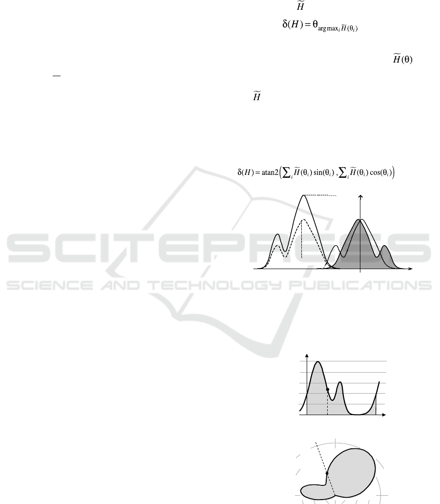
the characteristic direction of H and denote by (H):
H()  H((H ))
(17)
See Fig. 1. The normalizing transformation, t
H
, is
then the rotation about the origin with angle (H).
There are many ways to define (H). For example,
it may be set to the direction  in [0, 2) that
maximizes H():
(H ) 
argmax
i
H(
i
)
(18)
The approach is used in (Buck et al., 2010). However,
H is not normalizable if multiple directions maximize
H(). In practice, this means that the computed
characteristic direction—and, therefore, the
normalization procedure—is unreliable when
multiple histogram values are very close to the
maximum histogram value. The issue cannot be
ignored, as many man-made object pairs exhibit
symmetry and are ill-behaved.
Consider the centroid of the region defined by
the rectangular representation of H on an arbitrary 2-
long interval. (H) cannot be set to the x-coordinate
of that centroid, because it would depend on the
chosen interval. However, (H) can be set to the
angular coordinate of the centroid of the region
defined by the polar representation of H (Fig. 2b):


33
() atan2 ()sin(), ()cos()
ii i i
ii
HH H    

(19)
where atan2 is the two-argument variation of the
arctangent function.
Equation (19) seems overly complicated. A
similar but simpler approach is to see each pair (,
H()) as the polar coordinates of a vector and to
define the characteristic direction (H) as the
direction of the sum of all these vectors (Fisher,
1995):
(H)  atan2 H(
i
)sin(
i
)
i

, H(
i
)cos(
i
)
i


(20)
The histogram H is not normalizable if the
arguments of the atan2 function in (20) are both zero.
In practice, this means that the computed
characteristic direction is unreliable when the two
arguments are very close to zero. At any rate, an
object pair is far less likely to be ill-behaved with (20)
than with (18).
To address the issue with (18), we can also replace
H on the right-hand side with the histogram of
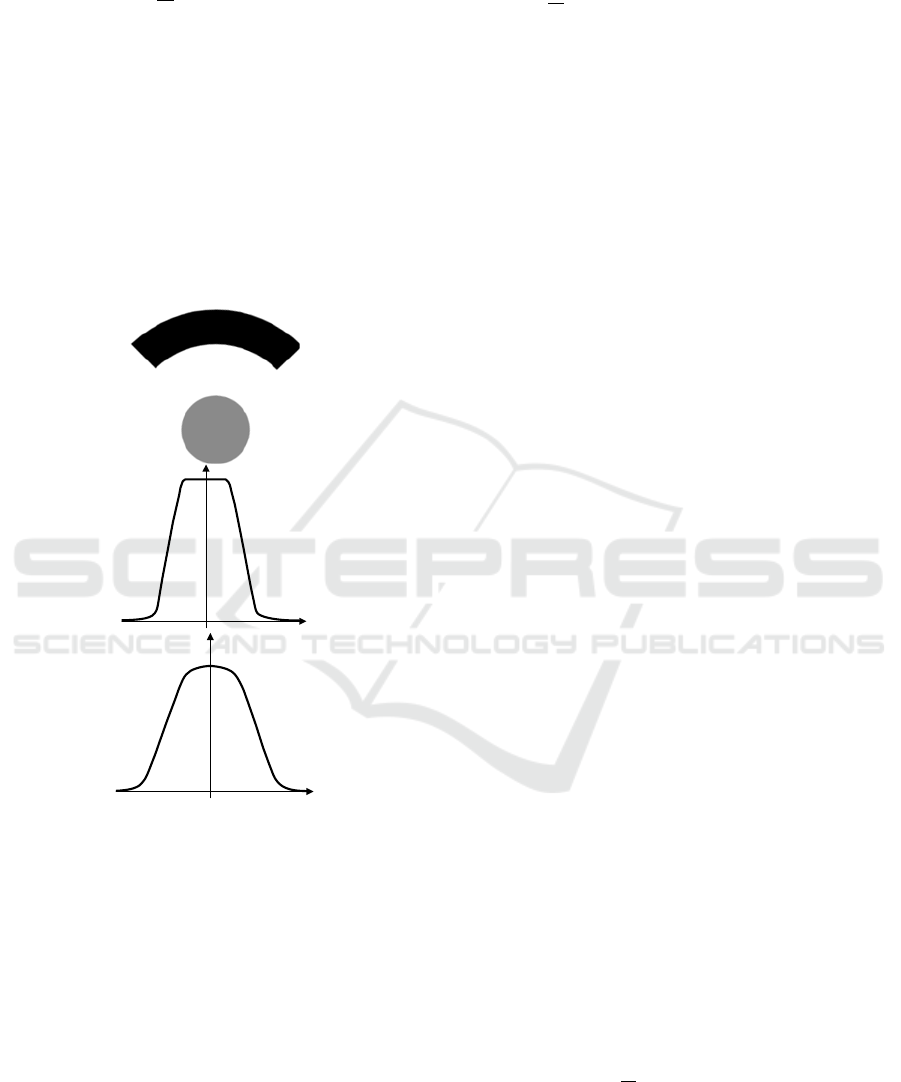
degrees of truth :
(21)
Assume H represents the relative position of two
objects A and B, i.e., H=h
AB
. The value is the
degree of truth of the proposition “A is in direction 
of B.” It belongs to [0,1], with 0 for false and 1 for
true.
is derived from H by categorizing forces into
contradictory, compensatory and effective forces
(Matsakis et al., 2001). Its particularity is that, in most
cases, only one direction maps to the maximum
degree of truth (Fig. 3). Note that (20) can be revised
the same way:
(22)
Figure 1: H
0
: original histogram. H
1
: after normalization
w.r.t. the scaling-translation group. H
2
: after normalization
w.r.t. direct similitudes. H
3
: after normalization w.r.t.
similitudes. Note that: (H
1
)=(H
2
)=(H
3
)=1,
(H
0
)=(H
1
),
(H
2
)=(H
3
)=0, (H
0
)=(H
1
)=(H
2
)=1, (H
3
)=+1.
(a)
(b)
Figure 2: (a) Region (in grey) defined by the rectangular
representation of some histogram H on the interval [0,2].
(b) Region (in grey) defined by the polar representation of
the same histogram.
H

0

H

0

/2
H
0
H
1
H
2
H
3

(
H
1
)

(
H
0
)
Normalization of the Histogram of Forces
633

Whatever the definition of the characteristic
direction:
(H)  0
(23)
Note that (21) (22) are used in (Skubic et al., 2004);
(Buck et al., 2013), respectively. In these papers,
however, the authors rely on another histogram of
degrees of truth, not derived from H alone; the
described procedures are, therefore, not
normalization procedures as defined in Section 3.1.
The procedure described in (Vaduva et al., 2013) is not
a proper normalization procedure either, since the
characteristic direction is derived from the objects that
produce the force histogram, not from the histogram
itself.
Figure 3: (a) Two objects A and B. (b) The corresponding
histogram of forces. (c) The histogram of degrees of truth
derived from the histogram of forces.
3.6 Normalization w.r.t. the Isometry
Group
The isometry group can be generated by the set of all
reflections, or by the set of all rotations (which
generate the direct isometry group) and the reflection
about the line in direction 0 that passes through the
origin. When applying an isometry to a pair of
objects, the corresponding histogram H is shifted along
the x-axis—see (2)—and mirrored about the y-axis if
the isometry is indirect—see (3). All this must be
counterbalanced: first, normalize the histogram w.r.t
the direct isometry group; then, consider mirroring the
resulting histogram about the y-axis. In the end:
H()  H((H )(H ))
,
(24)
where the characteristic orientation (H) of H is
either +1 (no mirroring) or 1 (mirroring). See Fig. 1.
The normalizing transformation, t
H
, is then the
rotation about the origin with angle (H), followed,
if (H) is 1, by the reflection about the line in
direction 0 that passes through the origin.
There are many ways to define (H). For
example, it may be set to +1 if
[0, ] [0, ]
(( ) ) (( ) )
ii
ii
HH HH
   

   


(25)
and to 1 if the other strict inequality holds. Note
that the left (resp. right) hand side of the inequality is
the area of the half histogram to the left (resp. right)
of the characteristic direction. H is not normalizable
w.r.t. the isometry group if it is not normalizable w.r.t.
the direct isometry group, or if the characteristic
orientation is undefined (i.e., neither (25) nor the
other strict inequality holds). In practice, the latter
means that the computed characteristic orientation—
and, therefore, the whole normalization procedure—
is unreliable when the two halves of the histogram on
each side of the characteristic direction have about the
same area.
Another way to define (H) is to consider the
characteristic directions of the half histograms
instead of their areas. In other words, (H) may be set
to +1 if

(
H
LEF
T
) <

(
H
R
IGH
T
)
(26)
and to 1 if the other strict inequality holds. H
LEFT
is
the histogram defined by H
LEFT
() = H((H)) if
[0,) and H
LEFT
() = 0 if [,2). Likewise,
H
RIGHT
is defined by H
RIGHT
() = H((H)+) if
[0,) and H
RIGHT
() = 0 if [,2).
We may also want to consider the characteristic
forces of the half histograms instead of their areas or
characteristic directions. In other words, (H) may be
set to +1 if

(
H
LEF
T
) <

(
H
R
IGH
T
)
(27)
and to 1 if the other strict inequality holds.
Whatever the definition of the characteristic
orientation, we have:
(H) 1
(28)
A
B
h
AB
h
AB
~
1
0
(b)
(c)
(a)
ICPRAM 2019 - 8th International Conference on Pattern Recognition Applications and Methods
634

3.7 Normalization w.r.t. the Direct
Similitude Group
The direct similitude group can be generated by
the set of all scalings (which generate the scaling-
translation group) and rotations (which generate the
direct isometry group). A normalization procedure
w.r.t. that group can be obtained as follows: first,
normalize the histogram w.r.t. the scaling-translation
group, then normalize the resulting histogram w.r.t.
the direct isometry group (or vice versa); compose the
two normalizing transformations (in any order). We
have:
H() 
1
(H)
H((H))
(29)
H is not normalizable w.r.t. the direct similitude
group if it is not normalizable w.r.t. the direct
isometry group.
3.8 Normalization w.r.t. the Similitude
Group
Refer to Section 3.7: delete the word “direct”
everywhere, replace “rotations” with “reflections”
and (29) with (30):
H() 
1
(H)
H((H)(H ))
(30)
4 EXPERIMENTS
In this section, we conduct various experiments to
evaluate the performance of and compare the
normalization procedures discussed in Section 3. The
objects and histograms considered in the experiments
are presented in Sections 4.1 and 4.2. The
experiments themselves are described in Section 4.3.
The results are shown and analyzed in Section 4.4.
4.1 Objects
Two sets of objects were considered in our
experiments. The first one, B1, is a map of 95
buildings (from downtown New York City) and the
second one, B2, is a map of 86 buildings. Both were
acquired through Google Maps. See Fig. 4. The two
sets represent cases that are somewhat opposite: the
distances between neighbour objects are about the
same in B1, but vary significantly in B2; most objects
have simple, regular shapes in B1, but have more
complex and varied shapes in B2.
One hundred pairs of neighbour objects were
chosen randomly from each set, with the constraint
that each object of the set must be in at least one pair.
4.2 Histograms
Each histogram computed in our experiments was
computed using n=360 evenly distributed directions.
The two most common types of histogram were
considered: the histogram of constant forces, i.e.,
r=0, and the histogram of gravitational forces, i.e.,
r=2. For the meaning of n and r, see Section 2.2.
As mentioned in Section 3.2, we need a way to
assess the similarity between two histograms. In our
experiments, we used the Tversky index (Pappis and
Karacapilidis, 1993). See (31). It is a number between
0 (completely dissimilar) and 1 (completely similar).
Several similarity measures for the comparison of
force histograms were examined in (Matsakis et al.,
2004), and the Tversky index appeared to be the most
appropriate measure for the task.
si m(H,

H ) 
min{H(
i
),

H (
i
)}
i

max{H(
i
), H (
i
)}
i


(31)
4.3 Description of the Experiments
Many normalization procedures have been presented
in Section 3. Finding the best ones comes down to
finding the best ways to define the characteristic
force, direction, and orientation of a histogram. Three
experiments were therefore designed. The general
idea is to find, within a map of buildings, two
buildings in a given relative position. The position is
specified by a query, which is like a very small map
with only two buildings.
The first experiment relies on the assumption that
the North is indicated on both the map and the query,
but the scale of the map, or of the query, is unknown.
In other words, the normalization procedures
considered in the experiment are w.r.t the scaling-
translation group, and the aim is to determine the best
way to define the characteristic force: is it through
(13), (14), or (15)?
1. For each object pair repeat the following 10 times:
1.1. Scale the two objects, using a scale factor 
chosen randomly between 1 and 5.
1.2. For each normalization procedure and type
of histogram:
1.2.1. Record the similarity between the normalized
histograms of the object pair before and after
transformation.
1.2.2. Let ' be the retrieved scale factor as per (10).
Record the scale ratio max{'/, /'} (it is greater
than or equal to 1).
Normalization of the Histogram of Forces
635

2. For each normalization procedure and type of
histogram, derive some statistics from these records (e.g.,
min, max, mean, standard deviation, percentile curves).
The second experiment relies on the assumption that
the scale is indicated on both the map and the
query, but the North is not. In other words, the
normalization procedures considered in the
experiment are w.r.t the direct isometry group, and
the aim is to determine the best way to define the
characteristic direction: is it through (18), (19), (20),
(21), or (22)? Steps 1.1 and 1.2.2 above are changed
to:
1.1. Rotate the two objects, using a rotation angle 
chosen randomly between 0 and 180.
1.2.2. Let ' be the retrieved rotation angle (between
180 and 180). Record the angle deviation
180|180|'|| (it is greater than or equal to 0).
The third experiment relies on the assumption that the
scale is indicated on both the map and the query, but
the North is not; moreover, the map may have been
flipped about an arbitrary axis. In other words, the
normalization procedures considered in the
experiment are w.r.t the isometry group, and the aim
is to determine the best way to define the characteristic
orientation: is it through (25), (26), or (27)?
1. For each object pair repeat the following 5 times:
1.1. Rotate the two objects, using a rotation angle
chosen randomly between 0 and 180.
1.2. For each normalization procedure and type of
histogram:
1.2.1. If the histograms of the object pair before and
after transformation have both the same characteristic
orientation, record a true negative (TN).
2. For each object pair, repeat the following 5 times:
2.1. Reflect the two objects; the reflection is about a line
whose direction is chosen randomly.
2.2. For each normalization procedure and type of
histogram:
2.2.1. If the histograms of the object pair before and
after transformation have different characteristic
orientations, record a true positive (TP).
3. For each normalization procedure and type of histogram,
indicate TN and TP.
In practice, the querier does not know the exact
shapes of the two buildings they are looking for; the
focus is on the relative position of the buildings, not
on their shapes. This is why each one of the three
experiments was run three times with the 100 object
pairs from B1, and three times with the 100 object
pairs from B2. The second and third times, polygonal
approximations of the objects—instead of the objects
themselves—were scaled, rotated or reflected. The
approximations were computed using Ramer-Douglas-
Peucker algorithm (Ramer, 1972) (Douglas and
Peucker, 1973), and were rougher the third times.
See Fig. 5.
4.4 Results
Tables 1 and 2 summarize the results for the
normalization procedures w.r.t the scaling-translation
group. The bold values in the tables are the best
results returned (highest average similarity and
lowest average scale ratio), and the underlined values
are the second best results. The results are best when
the characteristic force is defined using the centroid-
based approach; see (15). The similarities are almost
always the highest, and the scale ratios the lowest
(i.e., the retrieved scale factor is the most accurate).
This is true for both maps of buildings and both types
of histogram. There is no clear winner between the
max-based approach, (13), and the mean-based
approach, (14).
Tables 3 and 4 summarize the results for the
normalization procedures w.r.t the direct isometry
group. The results are best (highest similarities and
lowest angle deviations) when the characteristic
direction is chosen based on the vector sum of the
histogram of degrees of truth; see (22). The approach
based on the vector sum of the force histogram, (20),
comes very close second; it is the approach we
would recommend, as it is much simpler and faster.
The worst way to choose the characteristic direction
when normalizing a force histogram w.r.t the direct
isometry group is the argmax-based approach, (18).
Tables 5 and 6 summarize the results for the
normalization procedures w.r.t the isometry group.
When normalizing w.r.t the isometry group, we need
to first normalize w.r.t the direct isometry group
(Section 3.6); the characteristic direction was chosen
based on the vector sum of the force histogram, as
recommended above (Tables 3 and 4). The question
then is how to choose the characteristic orientation.
The results are best (highest numbers of true
positives and true negatives) with the characteristic
force approach, (27); the characteristic force was
computed using the centroid-based approach, as per
the results above (Tables 1 and 2). The characteristic
direction approach, (26), comes second. The worst
way to choose the characteristic orientation is the
approach based on the areas of the two halves of the
force histogram, (25). These results stand for both
maps of buildings and both types of histogram.
ICPRAM 2019 - 8th International Conference on Pattern Recognition Applications and Methods
636

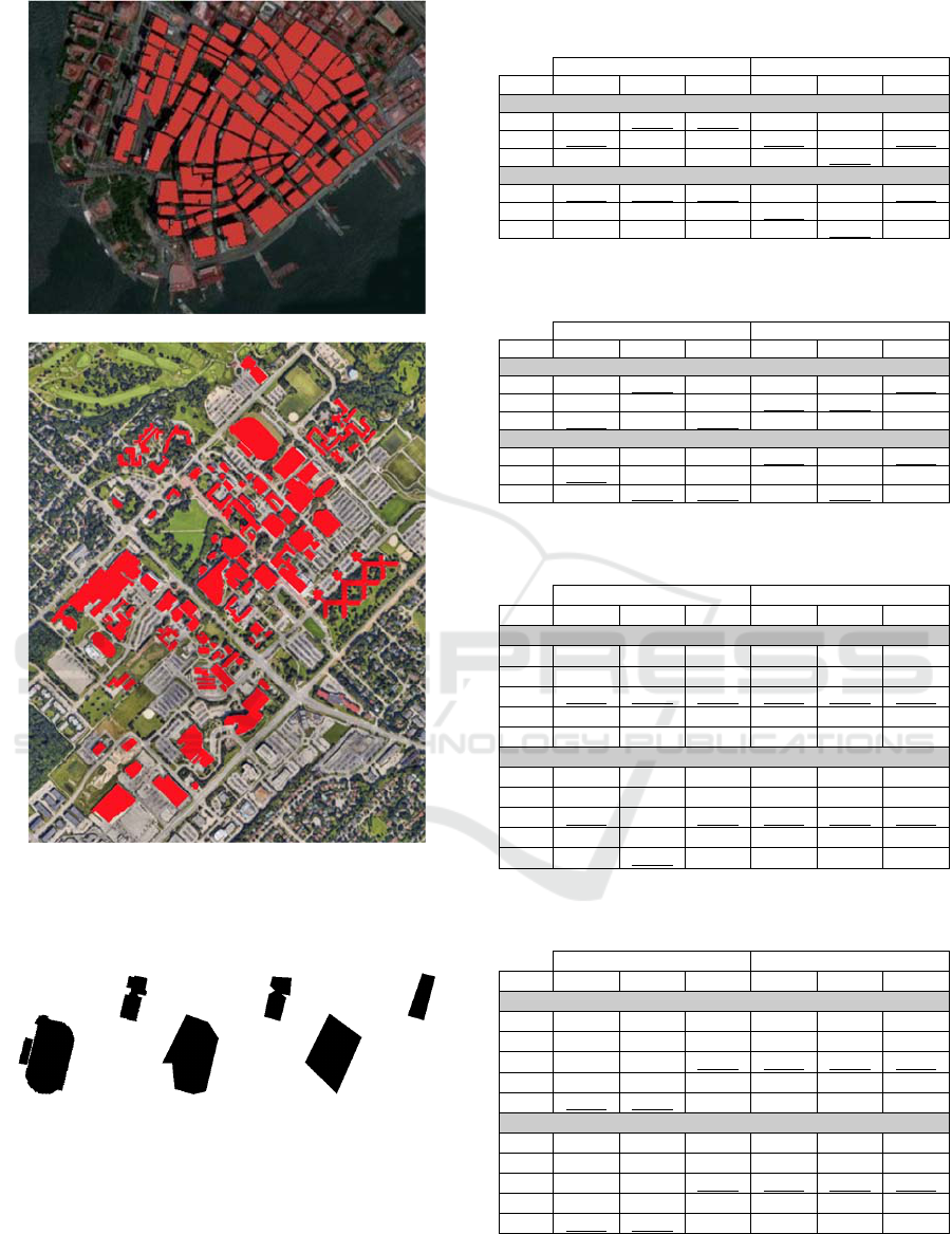
B1
B2
Figure 4: The two sets of objects used in the experiments.
Note that B1 was recorded as a 15001285 binary image,
and B2 as a 13061709 image.
P0 P1 P2
Figure 5: P0: no polygonal approximation of the objects,
i.e., original object pair (first run of the experiments with
B1 or B2). P1: polygonal approximation (second run). P2:
rougher polygonal approximation (third run).
Table 1: Results of normalizing the force histogram of type r
= 0 w.r.t the scaling-translation group.
B1 B2
P0 P1 P2 P0 P1 P2
average similarit
y
(
13
)
0.9987 0.9676 0.9532 0.9960 0.9276 0.8924
(14) 0.9988 0.9668 0.9531 0.9964 0.9317 0.8947
(
15
)
0.9988 0.9682 0.9545 0.9965 0.9315 0.8962
average scale ratio
(
13
)
1.0004 1.0210 1.0382 1.0012 1.0238 1.0494
(14) 1.0005 1.0269 1.0478 1.0012 1.0353 1.0571
(
15
)
1.0004 1.0205 1.0377 1.0010 1.0239 1.0465
Table 2: Results of normalizing the force histogram of type r
= 2 w.r.t the scaling-translation group.
B1 B2
P0 P1 P2 P0 P1 P2
avera
g
e similarit
y
(
13
)
0.9981 0.9692 0.9509 0.9953 0.9346 0.8866
(
14
)
0.9983 0.9686 0.9487 0.9958 0.9349 0.8856
(
15
)
0.9983 0.9701 0.9501 0.9958 0.9368 0.8891
avera
g
e scale ratio
(
13
)
1.0022 1.1026 1.1847 1.0042 1.1329 1.2622
(
14
)
1.0022 1.1269 1.2347 1.0042 1.1811 1.3210
(
15
)
1.0019 1.1033 1.1940 1.0036 1.1419 1.2561
Table 3: Results of normalizing the force histogram of type r
= 0 w.r.t the direct isometry group.
B1 B2
P0 P1 P2 P0 P1 P2
average similarity
(18) 0.9845 0.9145 0.8562 0.9703 0.8735 0.7952
(19) 0.9887 0.9272 0.8724 0.9741 0.8860 0.8275
(20) 0.9886 0.9276 0.8738 0.9748 0.8904 0.8330
(21) 0.9877 0.9256 0.8725 0.9738 0.8859 0.8209
(22) 0.9884 0.9278 0.8741 0.9755 0.8908 0.8334
average angle deviation
(18) 0.4504 1.3738 2.3920 0.3922 2.1481 4.3300
(19) 0.3300 0.7292 1.2361 0.3299 1.6419 2.2185
(20) 0.3366 0.6781 1.0684 0.3216 1.2542 1.7441
(21) 0.3562 0.8636 1.3523 0.3375 1.5833 2.7246
(22) 0.3414 0.6875 1.0643 0.3099 1.2095 1.6593
Table 4: Results of normalizing the force histogram of type r
= 2 w.r.t the direct isometry group.
B1 B2
P0 P1 P2 P0 P1 P2
average similarity
(18) 0.9771 0.8854 0.8261 0.9643 0.8559 0.7663
(19) 0.9888 0.8916 0.8346 0.9751 0.8789 0.7884
(20) 0.9892 0.8922 0.8365 0.9753 0.8812 0.7926
(21) 0.9896 0.8910 0.8360 0.9762 0.8776 0.7876
(22) 0.9893 0.8922 0.8367 0.9751 0.8814 0.7929
average angle deviation
(18) 0.7986 1.4829 2.5389 0.5872 3.9653 5.6347
(19) 0.3547 0.8801 1.3538 0.3481 1.9990 4.0156
(20) 0.3417 0.8378 1.0093 0.3412 1.4147 3.2392
(21) 0.3248 0.9016 1.1300 0.3283 1.6755 3.9143
(22) 0.3378 0.8449 0.9860 0.3380 1.3098 3.1818
Normalization of the Histogram of Forces
637

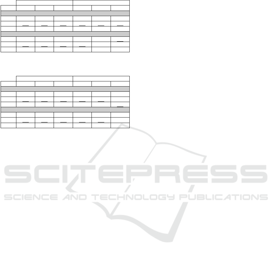
Table 5: Results of normalizing the force histogram of type r
= 0 w.r.t the isometry group.
B1 B2
P0 P1 P2 P0 P1 P2
true negatives
(
25
)
402 396 400 416 383 346
(26) 440 436 440 436 406 402
(
27
)
483 487 470 487 456 421
true
p
ositives
(
25
)
420 423 402 424 415 383
(26) 454 440 448 450 415 375
(
27
)
483 474 460 475 450 417
Table 6: Results of normalizing the force histogram of type r
= 2 w.r.t the isometry group.
B1 B2
P0 P1 P2 P0 P1 P2
true ne
g
atives
(
25
)
393 385 388 392 388 334
(
26
)
418 427 426 426 393 387
(
27
)
463 450 448 481 445 380
true
p
ositives
(
25
)
382 394 374 385 370 296
(
26
)
429 413 426 433 387 370
(
27
)
465 451 458 490 421 353
5 CONCLUSION
Making the histogram of forces invariant under
similitudes is achieved through a procedure called
normalization. Various normalization procedures
can be found in the literature, but they had not been
assessed or compared, and invariance under direct
similitudes only was actually achieved.
We have shown that the histogram of forces can
be made invariant under the similitude group or under
a subgroup of that group, and that any normalization
procedure to achieve such goal relies on one or more
of three values derived from the histogram: the
characteristic force, the characteristic direction, and
the characteristic orientation.
We have reviewed the existing procedures, we
have introduced new ones, and we have shown
through comparative experiments involving over
170,000 histogram computations or normalizations
that many of these new procedures outperform the
existing ones.
Making the histogram of forces invariant under
the affine group remains an unsolved problem, and
we will tackle it in future work. We will also
examine normalization procedures for other relative
position descriptors.
REFERENCES
A. R. Buck, J.M. Keller, M. Skubic, “A modified genetic
algorithm for matching building sets with the
histograms of forces,” IEEE Congress on
Evolutionary Computation (CEC), Proceedings, 1-7,
2010.
A. R. Buck, J.M. Keller, M. Skubic, “A memetic algorithm
for matching spatial configurations with the histogram
of forces,” IEEE Trans. on Evolutionary Computation,
17(4): 588-604, 2013.
M. Clement, C. Kurtz, L. Wendling, “Bags of spatial
relations and shapes features for structural object
description,” 23rd Int. Conf. on Pattern Recognition
(ICPR), Proceedings, 1994-9, 2016.
I. Debled-Rennesson, L. Wendling. “Combining force
histogram and discrete lines to extract dashed lines,”
20th Int. Conf. on Pattern Recognition (ICPR),
Proceedings, 1574-7, 2010.
D. Douglas, T. Peucker, “Algorithms for the reduction of
the number of points required to represent a digitized
line or its caricature,” The Canadian Cartographer,
10(2):112–22, 1973.
N. I. Fisher, Statistical Analysis of Circular Data,
Cambridge University Press, 1995.
M. Li, A. Stein, W. Bijker, Q. Zhan, “Urban land use
extraction from very high resolution remote sensing
imagery using a Bayesian network,” ISPRS J. of Pho-
togrammetry and Remote Sensing, 122:192-205, 2016.
P. Matsakis, J.M. Keller, O. Sjahputera, J. Marjamaa, “The
use of force histograms for affine-invariant relative
position description,” IEEE Trans. on Pattern Analysis
and Machine Intelligence, 26(1):1-18, 2004.
P. Matsakis, J.M. Keller, L. Wendling, J. Marjamaa, O.
Sjahputera, “Linguistic description of relative positions
in images,” IEEE Trans. on Systems, Man, and
Cybernetics, Part B, 31(4):573-88, 2001.
P. Matsakis, L. Wendling, J. Ni, “A General Approach to
the Fuzzy Modeling of Spatial Relationships,” In: R.
Jeansoulin, O. Papini, H. Prade, S. Schockaert (Eds.):
Methods for Handling Imperfect Spatial Information,
Springer-Verlag, 49-74, 2010.
M. Naeem, P. Matsakis, “Relative position descriptors: A
review,” 4th Int. Conf. on Pattern Recognition
Applications and Methods (ICPRAM), Proceedings,
286-95, 2015.
J. Ni, P. Matsakis, “An equivalent definition of the
histogram of forces: Theoretical and algorithmic
implications,” Pattern Recognition, 43(4):1607-17,
2010.
C. Pappis, N. Karacapilidis, “A Comparative Assessment
of Measures of Similarity of Fuzzy Values,” Fuzzy Sets
and Systems, 56(2):171-4, 1993.
U. Ramer, “An iterative procedure for the polygonal
approximation of plane curves,” Computer Graphics
and Image Processing, 1(3):244–56, 1972.
C.-R. Shyu, M. Klaric, G.J. Scott, A.S. Barb, C.H. Davis,
K. Palaniappan, “Geoiris: Geospatial information
retrieval and indexing system—content mining,
semantics modeling, and complex queries,” IEEE
Trans. on Geoscience and Remote Sensing, 45(4):839-
52, 2007.
ICPRAM 2019 - 8th International Conference on Pattern Recognition Applications and Methods
638

O. Sjahputera, J.M. Keller, “Scene matching using f-
histogram-based features with possibilistic c-means
optimization,” Fuzzy Sets and Systems, 158(3):253-69,
2007.
M. Skubic, D. Perzanowski, S. Blisard, A. Schultz, W.
Adams, M. Bugajska, D. Brock, “Spatial language for
human-robot dialogs,” IEEE Trans. on Systems, Man,
and Cybernetics, Part C, 34(2):154-67, 2004.
C. Vaduva, I. Gavat, M. Datcu, “Latent Dirichlet allocation
for spatial analysis of satellite images,” IEEE Trans. on
Geoscience and Remote Sensing, 51(5): 2770-86,
2013.
Normalization of the Histogram of Forces
639