Data-driven Autism Biomarkers Selection by using Signal Processing and
Machine Learning Techniques
Antonio Antovski
1
, Stefani Kostadinovska
1
, Monika Simjanoska
1
, Tome Eftimov
2
,
Nevena Ackovska
1
and Ana Madevska Bogdanova
1
1
Faculty of Computer Science and Engineering, Ss. Cyril and Methodius University,
Rugjer Boshkovikj 16, 1000 Skopje, Macedonia
2
Computer Systems Department, Jo
ˇ
zef Stefan Institute, Jamova cesta 39, 1000 Ljubljana, Slovenia
Keywords:
Autism, Gene Expression, Fractional Fourier Transform, Entropy, Machine Learning, Ranking, Biomarkers
Selection.
Abstract:
To analyze microarray gene expression data from homogeneous group of children diagnosed with classic
autism, a synergy of signal processing and machine learning techniques is proposed. The main focus of
the paper is the gene expression preprocessing, which relies on Fractional Fourier Transformation, and the
obtained data is further used for biomarker selection using an entropy-based method. This is a crucial step
needed to obtain knowledge of the most informative genes (biomarkers) in terms of their discriminative power
between the autistic and the control (healthy) group. The relevance of the selected biomarkers is tested using
discriminative and generative machine learning classification algorithms. Furthermore, a data-driven approach
is used to evaluate the performance of the classifiers by using a set of two performance measures (sensitivity
and specificity). The evaluation showed that the model learned by Naive Bayes provides best results. Finally,
a reliable biomarkers set is obtained and each gene is analyzed in terms of its chromosomal location and
accordingly compared to the critical chromosomes published in the literature.
1 INTRODUCTION
Autism is considered to be neurodevelopmental dis-
order, emerging from the early childhood. It is often
manifested by an impediment in personal, social, aca-
demic, or professional functioning. (Azizi, 2015)
Autism Spectrum Disorder (ASD) is characterized
by troubles with social interaction and communica-
tion, as well as by restricted and repetitive behavior.
The first signs of ASD occur in the first 18-30 months
of the child’s life (Baron-Cohen et al., 1992), and they
are of progressive nature. Globally, in 2015, the num-
ber of people who have been diagnosed with autism
is 24.8 million (Wikipedia, 2016).
Autism reflects on the brain information process-
ing and thus, on the way the neurons and the synapses
are linked between. However, there are not sufficient
number of research papers to confirm this hypothe-
sis. By now, it is confirmed that the autism has a
strong genetic basis that is complex and vague since
this disorder comes out of rare mutations with big ef-
fects and/or out of rare multigenomic interactions of
common gene variants (Yuen et al., 2017).
The enormous progress of the DNA microarrays
allowed the researchers to analyze the expression lev-
els of thousands of genes simultaneously. There
is a correlation between the different genes regula-
tion, meaning we have to consider the co-operability
among the genes in order to find the true character-
istics of a genome. In the literature, there is variety
of microarrays researches that usually include vari-
ous Machine Learning (ML) techniques to discover
the differences and characteristics of cancers, disor-
ders and/or diseases. However, the diagnosis of the
specific type of autism remains a challenge, since the
autism is represented by spectrum of disorders, in-
cluding Asperger’s syndrome, Pervasive developmen-
tal disorder, and Childhood disintegrative disorder.
In this paper, signal processing and ML methods
are fused to analyze microarray gene expression data
from homogeneous group of children diagnosed with
classic autism, excluding the autism with regression
and Asperger’s syndrome (Alter et al., 2011). The
focus of the paper is on the gene expression prepro-
Antovski, A., Kostadinovska, S., Simjanoska, M., Eftimov, T., Ackovska, N. and Bogdanova, A.
Data-driven Autism Biomarkers Selection by using Signal Processing and Machine Learning Techniques.
DOI: 10.5220/0007398902010208
In Proceedings of the 12th International Joint Conference on Biomedical Engineering Systems and Technologies (BIOSTEC 2019), pages 201-208
ISBN: 978-989-758-353-7
Copyright
c
 2019 by SCITEPRESS – Science and Technology Publications, Lda. All rights reserved
201

cessing as crucial step needed to obtain knowledge
of the most informative genes (biomarkers) in terms
of their discriminative power between the autistic and
the control (healthy) group. The biomarkers selec-
tion procedure relies on Fractional Fourier Transfor-
mation (FRFT) and on an Entropy - based method.
The relevance of the biomarkers is tested by several
discriminative and generative ML classification algo-
rithms. Furthermore, the performance of the classi-
fiers is ranked by a specific ranking approach that en-
ables the inclusion of multiple metrics when evaluat-
ing the classifier. At the end of the process, a reliable
biomarkers set is obtained and each gene is analyzed
in terms of its chromosomal location and accordingly
compared to the critical chromosomes published in
the literature.
The major contributions of the work presented in
this paper are multifold:
• Signal processing technique is shown to be ap-
plicative for gene expression data normalization;
• The preprocessing methods used allow proposi-
tion of multiple candidate biomarkers sets;
• The ML methods are used to find the most promis-
ing biomarkers set;
• Multiple ML discriminative and generative mod-
els are built for autism prediction and the gener-
ative approach is chosen as best (Naive Bayes),
achieving high sensitivity and specificity;
• Data-driven analysis is done to obtain reliable
choice for suitable biomarkers set;
• The biomarkers set is further analyzed and com-
pared to the literature.
The rest of the paper is organized as follows. In
Section 2 we present the published work related to our
problem. Sections 3 and 4 present the data used and
the methodology developed. The experiments and the
results are explained in Section 5. Finally, the conclu-
sion is given in the last Section 6.
2 RELATED WORK
ASD shows an extreme clinical heterogeneity, and
thus, it is very interesting for the researchers to in-
vestigate the disorders at genomic level.
Copy Number Variants (CNVs) are considered as
one of the main reasons for ASD. The triplication
of chromosome 15q11-q13, deletion on chromosome
9p24, and deletion on chromosome 3q29, are some of
the CNVs published in (Nava et al., 2014). Besides
these variants, the researchers succeeded in finding
the critical regions related to ASD. The work pub-
lished in (Philippi et al., 2005) summarize multiple re-
lated research papers and finds chromosome 16p to be
commonly discussed along with the PRKCB1 gene,
which is considered to be involved in the etiology of
the autism, but still cannot be proved.
As the connection between the CNVs and the
chromosomal alterations with the ASD is confirmed,
the genetic mutations often cover multiple genes, sin-
gle genes isomorphs, as well as regulatory elements,
e.g. the ASD - risk gene, PTCHD1-AS and combina-
tions of its mutations (Yuen et al., 2017).
Some other research papers refer to other genes
that might be related to the ASD, e.g. duplication
and/or deletion of the genes that are on the 22q11.2
chromosome. Also, there are new CNVs included,
obtained with deletion in the 18q22 region (Ceylan
et al., 2018).
A connection between the mitochondrial disfunc-
tion and ASD has been discovered by finding the
common mutations while investigating the patients’
mtDNA. Even though it has been concluded that the
mtDNA mutations are more common at ASD patients
rather than the controls, the mtDNA deletions are not
always related only to ASD, but there are other cases
where they are associated with alterations in genes
responsible for intergenomic communication (Varga
et al., 2018).
3 MATERIALS
The dataset used in this paper is obtained from the
NCBI database, identified as GSE25507 (Alter et al.,
2011). This dataset consists of 54613 probes and 146
samples in total, from which 82 refer to patients diag-
nosed with autism, and 64 controls, i.e. healthy sam-
ples. The platform for the initial execution of the ex-
periment is Affymetrix Human Genome U133 Plus 2
Array.
4 METHODOLOGY
The methodology proposed in this paper was inspired
by the work of Guo et al. (Guo et al., 2017) and
adapted to the problem at hand. The idea of applying
signal processing technique on autism gene expres-
sion data was challenging, since up to our knowledge,
none of the papers reported in the literature has ap-
plied such techniques on the autism problem before.
The methodology was developed by following the
classical ML procedure and fused with data-driven
BIOINFORMATICS 2019 - 10th International Conference on Bioinformatics Models, Methods and Algorithms
202

ranking method to find the best model and biomark-
ers set. We used Matlab for calculating FRFT coeffi-
cients and ranking the FRFT coefficients. For gener-
ating and evaluating the ML models we used Python.
Each step of the methodology is explained in the fol-
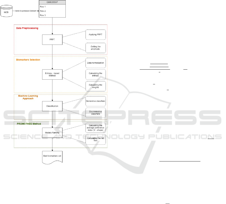
lowing subsections and depicted in Figure 1.
Figure 1: The methodology.
4.1 Data Preprocessing
Gene expression data are characterized with high di-
mensionality. In our case we are able to observe
54613 probes simultaneously. Choosing the represen-
tative features is crucial when building the classifica-
tion model, (Boulesteix et al., 2008), however, when
reducing the dimensionality, we have to be careful not
to lose any significant information that would lead to
a poor classification of new patients’ gene expression
data (Alkoot and Alqallaf, 2016).
Noise is a common issue when analyzing gene ex-
pression data and can be either of biological or tech-
nical nature. Therefore, normalizing the gene expres-
sion data before applying methods for knowledge ex-
traction is an essential step for reliable biomarkers set
selection. In this paper we use the application of the
Fractional Fourier Transformation (FRFT) as a gen-
eralized form of the standard Fourier Transformation
(FT) as proposed by Guo et al.(Guo et al., 2017). With
the FRFT we map the data from a spatial, or time do-
main into a frequency domain, obtaining the gene’s
amplitude and phase. FRFT can be thought of as a
linear operator defined with the following Equation
1:
f
p
(u) =
Z
+∞
−∞
f (t)K
p
(t, u)dt (1)
where K
p
(t, u) represents a kernel function defined as:
K
p
(t, u) =





A
α
exp[ jπ(cot α −2ut csc α + t
2
)], α 6= nπ
δ(u −t), α = 2nπ
δ(u +t), α = (2n ±1)π
and A
α
=
exp[−
−jπsgn(sin α)
4+ jα
2
]
|sin α|
1
2
, α =
pn
2
, n ∈ Z, δ(t) is the
Dirac function.
If α = 2nπ +
π
2
, FRFT is the standard FT, whereas
for each value 0 < α <
π
2
a rotated time series is pro-
duced, i.e., frequency representation of the signal.
The result of this transformation is a complex
number which can be plot on an Argand diagram.
From the Argand diagram, we then have the polar co-
ordinates of the complex number (modulus and argu-
ment), where the modulus matches the amplitude of
the complex number and the argument is the phase of
the complex number.
Let z = x + iy, where x, y ∈ R and i =
√
−1. The
amplitude can be obtained from the complex number
by using the following Equation 2:
|z| =
q
Real(z)
2
+ Imag(z)
2
(2)
where x is the real part of the complex number and y
is the imaginary part.
Some of the FRFT parameters are fixed, some are
calculated by equations, and some can accept a range
of real values that change the overall results. Consid-
ering the equation α =
pn
2
, it can be noticed that there
is a parameter p that does not have a predefined value.
Choosing different values for p affects the rotation of
the signal. Thus, we experiment with different values
for p and do FRFT for each probe of the gene expres-
sion dataset, mapping it in a vector of complex values
and hereupon calculate the amplitudes. The parame-
ter p differs from the p used in statistics.
4.2 Biomarkers Selection
As we obtained a normalized gene expression dataset,
we are interested in finding the most significant
Data-driven Autism Biomarkers Selection by using Signal Processing and Machine Learning Techniques
203

probes (genes). For this purpose we use the entropy
as a measure of randomness or disruption of a system.
This method is very useful in cases where we want to
add weights on some coefficients, or parameters. The
benefit of using the entropy is in its objectivity. Con-
sidered to be fixed, it weights the specified parameter
by using its quantity of information.
In this research, the entropy-based method is used
to estimate, i.e., to give specific weights to the ob-
tained FRFT coefficients, in order to find the ones
with the biggest quantity of information. The coef-
ficients with the biggest quantity of information are
selected to be biomarkers upon which an intelligent
model is built.
Let us have i samples and j FRFT coefficients,
where x
i j
is the j-th amplitude of the FRFT coeffi-
cient of the i-th sample. To eliminate the influence
among the coefficients, we normalize them by using
Equation 3:
r
‘
i j
=
x
i j
max{x
i j
}
, (i = 1, ..., m; j = 1, ..., n) (3)
and map them in range [0, 1] (Equation 4).
f
i j
=
r
‘
i j
∑
m
i=1
r
‘
i j
, (i = 1, ..., m; j = 1, ..., n) (4)
Hereupon, the entropy is calculated for each of the
coefficients by using the Equation 5:
H
j
= −
∑
m
i=1
f
i j
ln f i j
lnm
, (i = 1, ..., m; j = 1, ..., n) (5)
Finally, the weight of each coefficient is calculated
by using Equation 6:
w
j
=
1 −H
j
n −
∑
n
j=1
H
j
, (
n
∑
j=1
w
j
= 1; j = 1, ..., n) (6)
Following the advice of Guo et al. (Guo et al.,
2017), we ranked the probes according to their
weights and chose the top 300 (0.55% of all) to be
the most significant, referred to as biomarkers.
4.3 Machine Learning Approach
In order to test the relevance of the chosen biomark-
ers, we tested their discriminative power between
healthy and autistic patient’s gene expression data by
applying different machine learning methods. In or-
der to model the problem from different aspects, we
chose representative methods from both discrimina-
tive and generative approaches. All the classifiers
used the default parameters values. Three discrimi-
native classifiers were used as follows.
• Support Vector Machine (SVM). Two different
types of the SVM classifiers were used, Lin-
earSVM and NuSVM. The difference between
LinearSVM and NuSVM classifiers is in the type
of function used to separate the feature space.
LinearSVM uses linear function, and the NuSVM
classifier uses the radial basis kernel function.
• K - Nearest Neighbors (KNN). KNN is a non-
parametric method whose input consists of the k
closest training examples in the feature space. The
class of the new samples will be the same as the
class of the majority of its neighbors.
• Random Forest (RF). RF is an ensemble classifi-
cation method that uses multiple decision trees for
classifying a given sample. The advantage over
the decision trees is that the RF classifier avoids
overfitting over the training data.
Naive Bayes is used as a representative from the
generative approach. It is a probabilistic classifier
based on the Bayes’ Theorem.
Each of the classifiers was evaluated by using 10-
fold cross-validation method. This method groups the
data in 10 sets. In every step, one of these sets, that
hasn’t been chosen before, is chosen to be the test-
ing set and the others are used for training the model.
The overall result, for sensitivity, specificity and ac-
curacy, for every classifier represents the average of
the results obtained in every step of the 10-fold cross-
validation method.
The performance of the models was measured
by using the standard evaluation metrics for medical
problems. Sensitivity is used to evaluate how many of
the positive (autistic) samples were truly classified as
such. Specificity measures the model’s ability to rec-
ognize truly negative (healthy) samples. Eventually,
the overall accuracy for each classifier is obtained.
The calculation for each metric is given by the equa-
tions 7, 8 and 9, correspondingly,
sensitivity =
T P
T P + FN
(7)
speci f icity =
T N
T N + FP
(8)
accuracy =
T P + T N
T P + T N + FP + FN
(9)
where TP is the number of true positive predictions,
TN is the number of true negative predictions, FP is
the number of false positive predictions and FN is the
number of false negative predictions.
BIOINFORMATICS 2019 - 10th International Conference on Bioinformatics Models, Methods and Algorithms
204

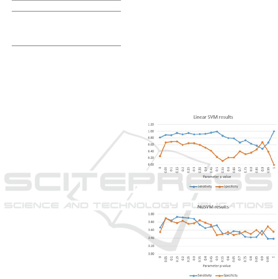
Table 1: Decision matrix.
Sensitivity (q
1
) Specificity (q
2
)
C
0
q
1
(C
0
) q
2
(C
0
)
C
0.05
q
1
(C
0.05
) q
2
(C
0.05
)
.
.
.
.
.
.
C
1
q
1
(C
1
) q
2
(C
1
)
4.4 PROMETHEE Method
To find the best value of p, which means to find the
best biomarkers set within each classifier, the conclu-
sion is made by fusing the result obtained for sen-
sitivity and specificity. The fusion is made follow-
ing the idea of PROMETHEE methods (Brans and
Mareschal, 2005). To compare the results obtained
for all p values within each classifier, and to select
the best p value, their results are organized into a
decision matrix (Table 1). The rows of the decision
matrix correspond to the same classifier trained with
different value of p, and the columns correspond to
the values obtained for the sensitivity and specificity.
First, a generalized preference function (Brans and
Mareschal, 2005) should be selected for each per-
formance measure. In our case, the V -shape gen-
eralized preference function is used for each perfor-
mance measure, where the threshold of strict prefer-
ence is set to the maximum difference that exists for
each preference measure from all pairwise compar-
isons according to that performance measure (Brans
and Mareschal, 2005). After that, the average pref-
erence index for each pair of meta-models should be
calculated, which gives information of global com-
parison between them using all performance mea-
sures. To rank the classifiers obtained for different
values of p, a net flow for each one needs to be calcu-
lated. It is a difference between a positive preference
flow and a negative preference flow of the classifier.
The positive preference flow gives information how a
given classifier is globally better than the other clas-
sifiers, while the negative preference flow gives the
information about how a given classifier is outranked
by all the other classifiers. This approach has been
already used for evaluation of multi-objective meta-
heuristic stochastic optimization algorithms regarding
a set of performance measures. More details about
the ranking approach and the equations for the net,
positive, and negative flow, can be find in (Brans and
Mareschal, 2005).
5 EXPERIMENTS AND RESULTS
Considering the data preprocessing explained in Sec-
tion 4.1, it can be noticed that the rotation of the
probes’ values in the FRFT method depends on the
parameter p. Providing different values for p, re-
sults in different weights for the probes in Section
4.2, meaning different probes might be ranked as top
300 and thus, different biomarkers sets will be cho-
sen. The best biomarker set is chosen according to
best results obtained as explained in Sections 4.3 and
4.4, and therefore, the best value for p.
For p, values are taken from the interval [0, 1]
in an ascending order with step of 0.05. Figures be-
low depict the sensitivity and the specificity metrics,
whereas the accuracy is omitted from the figures since
its information is included in the previous two.
Figure 2: LinearSVM Classifier.
Figure 3: NuSVM Classifier.
Figure 2 shows the sensitivity and specificity re-
sults obtained from the LinearSVM classifier. Con-
sidering the intention for obtaining both as close and
as high as possible sensitivity and specificity values
that explain the models ability to perform well on
both autistic and healthy samples, the most promising
values for the parameter p regarding the LinearSVM
model are in range [0.05-0.3]. For the other values
of the parameter p there is a decrease at both metrics,
especially at the specificity.
The most promising values for the parameter p at
the NuSVM model (figure 3) are shown to be from
Data-driven Autism Biomarkers Selection by using Signal Processing and Machine Learning Techniques
205

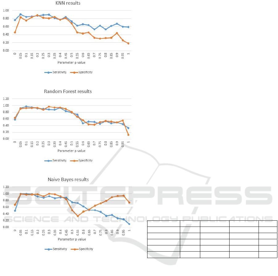
Figure 4: KNN Classifier.
Figure 5: Random Forest Classifier.
Figure 6: NaiveBayes Classifier.
0.05, up to 0.25. For the other values of the param-
eter p the models classification ability significantly
decreases and in some cases the specificity performs
better than the sensitivity which we find unfavorable
for our problem, meaning we prefer false positives
(autistic) rather than false negative (healthy) classi-
fications.
Figure 4 depicts the most promising values for the
parameter p at the KNN case to be all from 0.05, up
to 0.5. For values above 0.5, the model’s performance
decreases.
Figure 5 hows that RF behaves similarly to KNN,
again performing best for p in range [0.05-0.5]. How-
ever, when compared to all previously used discrim-
inative classifiers, it shows highest sensitivity and
specificity values.
Considering the generative Naive Bayes model,
the most promising values for the parameter p are
from 0.05, up to 0.45. For values above 0.45, the
model’s behavior is completely destabilized.
Given the figures, we have come to a conclusion
that at almost all models, the sensitivity and speci-
ficity is stable and satisfying when p varies in range
[0.05-0.5]. This conclusion, however, cannot tell on a
single best p value, meaning to find the best biomark-
ers set, and even more, on a single best classifier. For
that purpose, we propose the application of the data-
driven approach explained in Section 4.4 for finding
the best p value within a model, and afterwards find-
ing the best model that explains the relations in the
biomarkers set.
Table 3 presents the sensitivity and specificity for
all parameter values of p for each of the classifiers.
The bold values are found to be the best within each
classifier by using the PROMETHEE method. The
results provided in Table 2 present the best p parame-
ter results within each model. Eventually, the mod-
els are ranked and their status is shown in the last
column. From the results it can be concluded that
best biomarkers set is obtained when parameter p is
set to 0.05, for which the generative Naive Bayes
method achieved highest sensitivity and specificity
values. From the discriminative methods applied, RF
performed best when trained on biomarkers obtained
for p parameter set to 0.1.
Table 2: Ranking the classifiers.
Classifier Best p Sensitivity Specificity Rank
LinearSVM 0.15 0.95 0.70 4
NuSVM 0.05 0.90 0.90 3
KNN 0.05 0.90 0.84 5
RF 0.1 0.98 0.92 2
Naive Bayes 0.05 1 0.99 1
The biomarkers set relation to autism is further in-
spected by performing gene analysis to find their par-
ticular chromosomes locations. Table 4 presents the
chromosomes sorted by the number of biomarkers in-
side each of them.
When compared to the biomarker genes discov-
ered in the published literature, the following over-
lapping is found with four of the biomarkers we have
discovered:
• CD274 chromosome 9 location 9p24.1
• KMT2C chromosome 7 location 7q36.1
• KLF13 chromosome 15 location 15q13.3
• DOCK4 chromosome 7 location 7q31.1
Autism relation with chromosome 7 is already
proven before (Scherer et al., 2003; Cukier et al.,
2009; Ashley-Koch et al., 1999) and in the recent
BIOINFORMATICS 2019 - 10th International Conference on Bioinformatics Models, Methods and Algorithms
206

Table 3: Ranking the best biomarker sets within each classifier.
LinearSVM NuSVM KNN RF Na
¨
ıve Bayes
p Sensitivity Specificity Sensitivity Specificity Sensitivity Specificity Sensitivity Specificity Sensitivity Specificity
0 0.81 0.26 0.67 0.55 0.77 0.46 0.58 0.63 0.50 0.67
0.05 0.89 0.66 0.90 0.90 0.90 0.84 0.91 0.91 1.00 0.99
0.1 0.88 0.69 0.84 0.82 0.84 0.75 0.98 0.92 1.00 0.97
0.15 0.95 0.70 0.93 0.78 0.85 0.84 0.95 0.93 0.99 0.98
0.2 0.90 0.60 0.92 0.83 0.87 0.89 0.92 0.94 0.92 0.98
0.25 0.95 0.65 0.90 0.76 0.89 0.82 0.90 0.88 0.89 0.93
0.3 0.91 0.65 0.89 0.77 0.90 0.81 0.88 0.96 0.92 1.00
0.35 0.91 0.59 0.74 0.85 0.82 0.84 0.87 0.94 0.87 0.98
0.4 0.92 0.51 0.65 0.78 0.77 0.77 0.93 0.94 0.89 0.92
0.45 0.96 0.42 0.68 0.74 0.84 0.82 0.83 0.90 0.88 0.84
0.5 0.99 0.24 0.72 0.48 0.73 0.68 0.79 0.81 0.75 0.51
0.55 0.86 0.12 0.52 0.50 0.63 0.45 0.73 0.67 0.72 0.34
0.6 0.80 0.21 0.49 0.56 0.66 0.43 0.47 0.56 0.62 0.47
0.65 0.79 0.22 0.58 0.48 0.64 0.46 0.52 0.43 0.51 0.53
0.7 0.66 0.40 0.55 0.51 0.53 0.32 0.51 0.43 0.51 0.65
0.75 0.73 0.32 0.44 0.57 0.62 0.30 0.45 0.50 0.46 0.72
0.8 0.63 0.36 0.42 0.50 0.54 0.31 0.54 0.54 0.34 0.79
0.85 0.57 0.46 0.43 0.60 0.61 0.32 0.47 0.52 0.37 0.90
0.9 0.48 0.67 0.58 0.49 0.67 0.44 0.50 0.49 0.27 0.94
0.95 0.66 0.39 0.38 0.70 0.60 0.26 0.44 0.55 0.24 0.94
1 1.00 0.00 0.39 0.56 0.59 0.18 0.32 0.12 0.10 0.74
Table 4: Number of biomarker genes in each chromosome.
Chromosome Number of genes Genes
1 31
GBP1, ISG15, GBP5, ADAMTSL4, ASPM, CDC20,
C1QB, C4BPA, IFI44, THRAP3, DTL, UTS2, IFI44L, PTGS2, ATF3, C1QA, G0S2,
TACSTD2, IFI6, RAVER2, C1QC, GBP5, FCGR1B, CCL3L3
14 16
IFI27, EIF5, DLGAP5, RNASE3, RNASE2,
IGHV3-9, FOS, IGHV4-61, IGHD, IGHV3-7, IGHV4-61, IGHV1-69, IGHV3-23, IGHEP1,
IGHV3-72, IGHD
11 15
TRIM6, BATF2, NUMA1, MALAT1, FOLR3,
SERPING1, SF1, HBG2, CD3E, MMP8, NEAT1
17 15
TOP2A, EIF1, RP11-798G7.6, SOCS3, MXRA7,
CCL8, CCL2, RNF213, CCL23, CD7, XAF1, CDC6, SEPT4
10 13
SMC3, ANKRD22, KIF11, IFIT1, CDK1, CEP55,
NEBL, ZWINT, MCM10, IFIT3, IFIT2
2 13
SPATS2L, NR4A2, PLEKHB2, MXD1, RSAD2,
RRM2, CMPK2, RP11-373D23.2, CYP26B1
4 11
CXCL10, IL8, SPP1, EREG, BOD1L1, HERC5,
ANXA3, RAPGEF2, CXCL5, CXCL1
19 10
CEACAM8, UHRF1, TINCR, CD22, RETN, CD177,
FOSB, FCAR, LENG8
6 9
RNU6-1016P, HLA-DQA1, SOD2, PHACTR2,
CRISP3, TREML4, ETV7, ATXN1
5 8
FST, HBEGF, AC008964.1, EGR1, CD74,
CENPK, DUSP1
7 8
PSPH, KMT2C, AOC1, DOCK4, SAMD9L, NAMPT,
IFRD1, TMEM176B
8 8
ERG3, NKX3-1, DEFA4, ERICH1-AS1, MYOM2,
LY6E, PBK, IDO1
12 7
OAS3, OSBPL8, OASL, RP11-476D10.1,
A2M-AS1, C12ORF79
15 7
PKM, IGF1R, THBS1, CCNB2, IQGAP1,
KIAA0101, KLF13
22 7
IGLV3-10, IGLV4-60, IGLV3-25, FAM118A,
APOBEC3B, IGLV7-43, OSM
20 6 TPX2, PI3, TUBB1, RBM39, SIGLEC1
3 6 LAMP3, KIF15, GPR128, LTF, MBNL1, CPA3
9 5 CD274, TLN1, ORM1, ORM2, LCN2
18 4 TYMS, MBP, ZCCHC2
13 3 EPSTI1, OLFM4
21 3 MX1, ITGB2, SON
16 2 CYB5B, PRSS33
Data-driven Autism Biomarkers Selection by using Signal Processing and Machine Learning Techniques
207

literature (Klein-Tasman and Mervis, 2018), as well
as the chromosome 15 (Cooper et al., 2011; Sanders
et al., 2011; Sieg and Karl, 1990; Battaglia, 2008).
6 CONCLUSIONS
This paper proposes a methodology that is a fusion of
multiple different techniques with the aim to discover
a reliable biomarker set for autism recognition. Signal
processing technique is used to normalize the gene ex-
pression dataset, and a combination with the entropy-
based method is used to obtain different biomarkers
sets. The reliability of the biomarkers sets is mea-
sured by following standard ML approach including
discriminative and generative classification methods.
In order to find the best model, and therefore, the best
biomarkers set, a specific ranking method is applied.
The biomarkers set is further analyzed and compared
with the published literature. The results confirm a
relation between the biomarkers and the disorder in-
vestigated.
REFERENCES
Alkoot, F. M. and Alqallaf, A. K. (2016). Investigating ma-
chine learning techniques for the detection of autism.
Alter, M. D., Kharkar, R., Ramsey, K. E., Craig, D. W.,
Melmed, R. D., Grebe, T. A., Bay, R. C., Ober-
Reynolds, S., Kirwan, J., Jones, J. J., et al. (2011).
Autism and increased paternal age related changes in
global levels of gene expression regulation. PloS one,
6(2):e16715.
Ashley-Koch, A., Wolpert, C. M., Menold, M. M., Zaeem,
L., Basu, S., Donnelly, S. L., Ravan, S. A., Powell,
C. M., Qumsiyeh, M. B., Aylsworth, A., et al. (1999).
Genetic studies of autistic disorder and chromosome
7. Genomics, 61(3):227–236.
Azizi, Z. (2015). What is autism?
Baron-Cohen, S., Allen, J., and Gillberg, C. (1992). Can
autism be detected at 18 months?: The needle, the
haystack, and the chat.
Battaglia, A. (2008). The inv dup (15) or idic (15) syndrome
(tetrasomy 15q). Orphanet journal of rare diseases,
3(1):30.
Boulesteix, A.-L., Strobl, C., Augustin, T., and Daumer, M.
(2008). Evaluating microarray-based classifiers: an
overview.
Brans, J.-P. and Mareschal, B. (2005). Promethee methods.
In Multiple criteria decision analysis: state of the art
surveys, pages 163–186. Springer.
Ceylan, A. C., Citli, S., Erdem, H. B., Sahin, I., Arslan,
E. A., and Erdogan, M. (2018). Importance and usage
of chromosomal microarray analysis in diagnosing in-
tellectual disability, global developmental delay, and
autism; and discovering new loci for these disorders.
Cooper, G. M., Coe, B. P., Girirajan, S., Rosenfeld, J. A.,
Vu, T. H., Baker, C., Williams, C., Stalker, H., Hamid,
R., Hannig, V., et al. (2011). A copy number varia-
tion morbidity map of developmental delay. Nature
genetics, 43(9):838.
Cukier, H. N., Skaar, D. A., Rayner-Evans, M. Y., Konidari,
I., Whitehead, P. L., Jaworski, J. M., Cuccaro, M. L.,
Pericak-Vance, M. A., and Gilbert, J. R. (2009). Iden-
tification of chromosome 7 inversion breakpoints in
an autistic family narrows candidate region for autism
susceptibility. Autism Research, 2(5):258–266.
Guo, Z., Xin, Y., and Zhao, Y. (2017). Cancer classification
using entropy analysis in fractional fourier domain of
gene expression profile.
Klein-Tasman, B. P. and Mervis, C. B. (2018). Autism spec-
trum symptomatology among children with duplica-
tion 7q11. 23 syndrome. Journal of autism and devel-
opmental disorders, 48(6):1982–1994.
Nava, C., Keren, B., Mignot, C., Rastetter, A., Chantot-
Bastaraud, S., Faudet, A., Fonteneau, E., Amiet, C.,
Laurent, C., Jacquette, A., et al. (2014). Prospective
diagnostic analysis of copy number variants using snp
microarrays in individuals with autism spectrum dis-
orders.
Philippi, A., Roschmann, E., Tores, F., Lindenbaum, P.,
Benajou, A., Germain-Leclerc, L., Marcaillou, C.,
Fontaine, K., Vanpeene, M., Roy, S., et al. (2005).
Haplotypes in the gene encoding protein kinase c-
beta (prkcb1) on chromosome 16 are associated with
autism.
Sanders, S. J., Ercan-Sencicek, A. G., Hus, V., Luo, R.,
Murtha, M. T., Moreno-De-Luca, D., Chu, S. H.,
Moreau, M. P., Gupta, A. R., Thomson, S. A., et al.
(2011). Multiple recurrent de novo cnvs, including
duplications of the 7q11. 23 williams syndrome re-
gion, are strongly associated with autism. Neuron,
70(5):863–885.
Scherer, S. W., Cheung, J., MacDonald, J. R., Osborne,
L. R., Nakabayashi, K., Herbrick, J.-A., Carson, A. R.,
Parker-Katiraee, L., Skaug, J., Khaja, R., et al. (2003).
Human chromosome 7: Dna sequence and biology.
Science, 300(5620):767–772.
Sieg, M. and Karl, G. (1990). Neurodevelopmental disor-
ders associated with chromosome 15. Jefferson Jour-
nal of Psychiatry, 8(2):5.
Varga, N.
´
A., Pentel
´
enyi, K., Balicza, P., G
´
ezsi, A.,
Rem
´
enyi, V., H
´
arsfalvi, V., Bencsik, R., Ill
´
es, A.,
Prekop, C., and Moln
´
ar, M. J. (2018). Mitochondrial
dysfunction and autism: comprehensive genetic anal-
yses of children with autism and mtdna deletion.
Wikipedia (2016). Autism.
https://en.wikipedia.org/wiki/Autism. Accessed
on 10.08.2018.
Yuen, R. K., Merico, D., Bookman, M., Howe, J. L., Thiru-
vahindrapuram, B., Patel, R. V., Whitney, J., Deflaux,
N., Bingham, J., Wang, Z., et al. (2017). Whole
genome sequencing resource identifies 18 new candi-
date genes for autism spectrum disorder.
BIOINFORMATICS 2019 - 10th International Conference on Bioinformatics Models, Methods and Algorithms
208