
Improvements in the Current Brazil's Energy Dispatch Optimization:
Load Forecast and Wind Power
Gheisa Roberta Telles Esteves
1
, Paula Medina Maçaira
1
, Fernando Luiz Cyrino Oliveira
1
,
Gustavo Amador
2
and Reinaldo Castro Souza
1
1
Pontifical Catholic University of Rio de Janeiro - PUC-Rio, Rua Marquês de São Vicente, 225, Edifício Cardeal Leme,
9th Floor – Gávea, Rio de Janeiro, Cep: 22451-900, Brazil
2
CTG Brasil, R. Funchal, 418 - Vila Olimpia, São Paulo, SP, 04551-060, Brazil
Keywords: Load Demand Forecasting, Net Demand, Wind Power Generation Forecasting, and Energy Dispatch
Optimization.
Abstract: In the last years, Brazil has been passing through some significant changes into its electricity matrix, where
natural gas, wind power and other renewables sources are increasing its share on power generation. Those on
going changes represent a challenge to power generation dispatch, demanding improvements and major
changes on its management and optimization, especially due to growing levels of wind power generation.
From the power demand perspective, the use of too optimist power demand forecasts for energy planning and
dispatch optimization purposes affects it directly. This article intends to address those two issues, as it
proposes an alternative model to forecast electricity demand and conceives a procedure to integrate wind
power generation on the power dispatch model currently used in Brazil. The article study the Brazilian
Northeast region as it is where most of the wind power farms are located. Power demand forecasts are obtained
via electricity consumption forecasts made using Autoregressive Distributed Lag – ADL models, considering
macroeconomics perspectives to estimate it. To integrate wind power integration on the actual dispatch model,
the Markov Chain Monte Carlo method – MCMC was used to simulate wind power generation and calculate
the net power demand, which was considered in the dispatch model.
1 INTRODUCTION
In the last years, Brazil has been passing through
some significant changes into its electricity matrix
which itself represents a challenge to the dispatch
management and optimization. Renewables like wind
and solar generation are gaining space and
improvements into the actual dispatch model are
necessary to produce results that are more reliable.
Challenges also exists from the power demand point
of view to better represent the future perspective of
this variable, which also, indirectly, affects the
dispatch optimization and management. Those are the
two main issues considered in this article: provide an
alternative to the actual electricity demand forecasts
applied into the dispatch model and conceive a
procedure to introduce wind power generation into
the dispatch model.
1.1 Dispatch Optimization
Brazil has one of the cleanest electricity matrix in the
world, but aiming to better diversify it and due to
other environmental issues, other renewables (besides
from the hydropower generation) are gaining space
and thermal generation is migrating to natural gas.
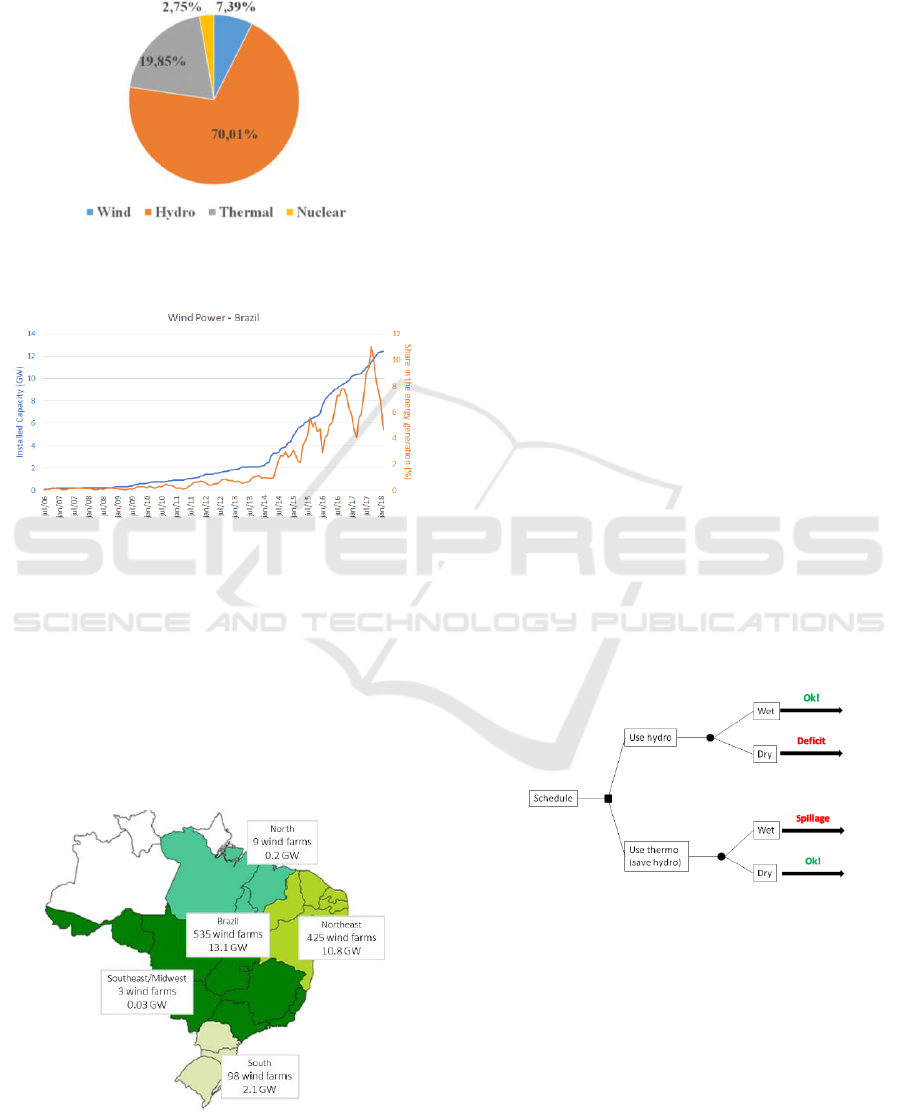
Figure 1 presents power generation matrix in 2017,
where around 42,3 thousand gigawatts are generated
through wind, being responsible for 7.39% of the
electricity generation (ONS, 2018). In 2015, wind
power had a share of just 3.90% of the electricity
generation. Observing the wind power generation and
its installed capacity numbers, for the last 10 years, it
possible to notice its constant growth, where in
January 2018, reached a total installed capacity of 12
GW (Figure 2).
Moreover, in the newer future, wind power tends to
keep increasing both its share in the Brazilian
electricity matrix (installed capacity) and its
generation share. Therefore, the actual power
398
Esteves, G., Maçaira, P., Oliveira, F., Amador, G. and Souza, R.
Improvements in the Current Brazil’s Energy Dispatch Optimization: Load Forecast and Wind Power.
DOI: 10.5220/0007400103980405
In Proceedings of the 8th International Conference on Operations Research and Enterprise Systems (ICORES 2019), pages 398-405
ISBN: 978-989-758-352-0
Copyright
c
2019 by SCITEPRESS – Science and Technology Publications, Lda. All rights reserved
dispatch model used in Brazil must be adapted to be
able to better represent this new configuration and to
produce more reliable results.
Source: Brazilian Power System Operator (ONS)
Figure 1: Brazilian Power Generation Matrix – 2017.
Source: Brazilian Power System Operator (ONS)
Figure 2: Wind Power Installed Capacity and Generation.
When it comes to wind power plants localization,
most of them are located on Brazilian northeast
region, where the environmental conditions are most
suitable (ANEEL). Figure 3 presents the installed
capacity per region and it is possible to notice that
almost 82.44% is located on the northeast and that´s
the main reason why our study focus the analysis in
this region.
Source: Brazilian Regulatory Authority (ANEEL)
Figure 3: Wind Power Farms Sites.
It is also important to mention that in Brazil, wind
power generation has a regime that is complementary
with hydroelectric generation. Therefore, in the dry
season wind power generation is able to fulfill the gap
left by hydropower generation decrease. This benefits
countries like Brazil that have most of its power
provided by hydropower. It also helps the country to
fulfill its greenhouse gas emissions targets.
As one of the article main purposes is to provide a
procedure to introduce wind power generation on the
Brazilian dispatch model, might be important to give
a brief overview of the power dispatch optimization
decision-making occurs. To manage the Brazilian
power sector, the system operator have to decide
whether to use all the water available in the present
moment or to save it for the future (Oliveira, 2015).
In other words, it is mainly a decision between
dispatching hydroelectric or thermal plants.
As can be seen in Figure 4, wind power generation is
not considered in the decision-making process.
Actually, to consider wind power generation in some
way, the system operator discounts the amount of
wind power generation forecasted deterministically
from the power demand considered in the decision-
making process. Therefore, the dispatch model uses a
net demand (power demand discounted the amount of
wind power generation forecasted), estimated
deterministically. In the article, we propose the use of
stochastic wind power simulations, calculated via
Markov Chain Monte Carlo (MCMC), as an
alternative method to estimate the net demand. This
represents the first step towards the conception of a
hydrothermal-wind dispatch model.
Figure 4: Power Dispatch Optimization.
1.2 Power Demand Modelling
As mentioned in Subsection 1.1, the net demand is
obtained taking from the power demand forecasted
the amount of wind power generated. Therefore,
power demand forecasts also have considerable
impacts on the results obtained during the decision-
making and the dispatch optimization process. Thus,
the more accurate the forecasts considered the better.
Inaccurate forecasts might give wrong price signals
Improvements in the Current Brazil’s Energy Dispatch Optimization: Load Forecast and Wind Power
399
or power dispatch signalizations to stakeholders
(Oliveira, 2015).
Nowadays, the Brazilian dispatch model consider
deterministic power demand forecasts instead of
probabilistic forecasts or even scenarios forecasts.
This article provides power demand scenarios using
electricity consumption forecasts conceived using
Additive Distributed Lags – ADL models. The use of
ADL models enables the use of explanatory variables
into the model. Three alternative scenarios (baseline,
optimist and pessimist) are elaborated.
1.3 Article Structure
The article has four sections including the
introduction. The second section contains the
methodology used both to the power dispatch
modelling and to the power demand forecasting.
Section 3 presents the results derived from the power
demand forecasting, wind power simulation and net
demand forecasts. It also contains the dispatch
optimization results considering both the actual
model used by the system operator and four
alternative scenarios. Section 4 contains the major
conclusions derived from both analyses.
2 METHODOLOGY
2.1 Load Forecasting
Monthly power demand scenarios were conceived
using monthly electricity consumption forecasts,
which were elaborated using Autoregressive
Distributed Lag - ADL modelling. The forecasts were
made by subsystem, on a monthly basis, for four years
ahead. The following mathematical equation
represents the ADL model:
(1)
Where:
: Dependent variable;
: Explanatory variables;
and
,
are finite
order lag polynomials with degree
: White noise.
ADL enables to model relationship between
independent and dependent variables and, in this
article, variables like income, gross domestic product
- GDP, retail sales, tariffs, temperature and rainfall
were used as explanatory variables. The electricity
consumption forecasts were made for each consumer
class; thus, a procedure was used to obtain power
demand forecasts scenarios from the electricity
consumption forecasts scenarios.
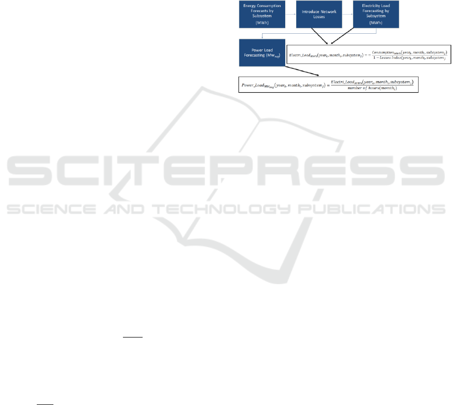
Figure 5 contains a flowchart of the procedure.
Initially, network losses are added on the monthly
consumption forecasts, generating monthly
electricity load forecasts. Then the monthly electricity
load forecasts are transformed into monthly power
demand forecasts.
Figure 5: Power Demand Scenarios Calculation.
The power demand forecasts and the official forecasts
(named NEWAVE) are evaluated via Mean Absolute
Percentage Error – MAPE to verify if the scenarios
conceive provides more accurate forecasts than the
ones considered by the system operator.
2.2 Wind Power Generation and Net
Demand
Before presenting the wind power generation
forecasts method and net demand estimation, a brief
overview is given of how wind power generation is
considered nowadays on the dispatch model.
The dispatch model considers wind power generation
together with, the so-called, non-simulated plants,
which are power plants that power generation are
added into the dispatch model deterministically. All
of them are taken into account on the dispatch model
through the net demand. The net demand is the
demand to be fulfilled in the dispatch optimization
and corresponds to the difference between the total
demand to be attended and the non-simulated plants
generation.
(2)
To estimate the wind power generation, stochastic
simulation is used and then these results are used to
calculated the net demand. This represents a different
where the net demand is calculated using historic wind
ICORES 2019 - 8th International Conference on Operations Research and Enterprise Systems
400

power generation data.
In our study, an analytical method of frequency and
duration is applied to combine wind power generation
and power demand to estimate the net demand. The
analytical method uses Markov chain and discrete
convolution techniques. This procedure was
conceived based on Almutairi et al (2016) study.
Figure 6 presents a procedure based on three steps
(historical data, MCMC model and Net Demand
Model) elaborated to treat wind power generation on
a stochastic manner.
Figure 6: Procedure Step by Step.
2.2.1 Historical Data
Papaefthymiou and Klöckl (2008) understand that a
stochastic model based on wind power generation is
more reliable and have more advantages than models
based on wind speed data. Therefore, in this study,
historical data of wind power generation is used.
Historical data for wind speed was obtained through
the Climate Forecast System Reanalysis - CFSR
(Saha et al., 2011) and as it enables the data gathering
by geographic coordinates (using a spatial resolution
between 0.25º to 0.25º), it was possible to associate a
wind speed data to each wind farm located on the
northeast region.
The wind speed data gathered was transformed into
wind power generation using turbine parameters from
each wind farm. The following parameters were
considered: turbine model, number of turbines,
average height and wind power load curve. More
information about this data is available at the
Regulatory Authority - ANEEL, the System Operator
- ONS and manufactures website.
Height correction errors were considered to relate the
wind speed gathered with each wind farm. The
correction is made using the following equation.
(3)
Where:
: Height correction factor;
: Turbine height;
: Measurement height associated with the wind
farm .
Wind power load curve associates a wind power to a
certain wind speed, therefore using the height
correction factor is possible to transform the wind
speed data
on wind power using the wind
power load curves.
2.2.2 Markov Chain Monte Carlo Model
The Markov Chain Monte Carlo - MCMC modelling
is divided into seven steps, explained below.
1. Aplication of k-means clustering techniques
(MacQueen, 1967) to transform the wind power data
(
into a finite number of states (
):
it is important to emphasize the in the end of the k-
means clustering the wind power calculated is
replaced by the centroids from the clusters where they
belong;
2. Calculates Markov Chain transition matrices
(
) where each row ends with 1: the transition
matrices are calculated for each month and have
dimension;
3. Calculate the cumulative probability transition
matrices where each row ends with 1: calculate the
transition probability (
) from the state to the
state , for all the matrix elements;
4. Select the initial state i randomly;
5. Produce a random value between 0 and 1 by
uniform random number generator;
6. Select the next state by comparing the value of a
random number with the elements of the ith row of
the cumulative probability transition;
7. Repeat steps 5 and 6 until the required hourly
wind power data is simulated.
2.2.3 Net Demand
To add the wind power generation into the Brazilian
hydrothermal dispatch model, it is crucial to have all
the data from the wind farms available. Consider that
there are wind farms on a certain database, each one
of them with a certain installed capacity (
,
). The wind farm share is calculate dividing
the wind farm installed capacity by the wind power
installed capacity considering all wind power
producers.
(4)
For example, if a certain wind power generator starts
its operation at day , month and year , all the
wind power generation simulated before this data
must be discounted from
.Concerningthe ca-
Improvements in the Current Brazil’s Energy Dispatch Optimization: Load Forecast and Wind Power
401

pacity and availability factor, as there is no
information about this matter for each wind farm,
historical data for one-year monthly generation is
used to calibrate the forecasted values. In other
words, for a month , o correction factor
is
calculated as following.
(5)
To start the net demand calculation, data from hourly
power demand forecasts are necessary. Due to the
lack of official information about hourly load curves
for Brazil, a standard load curve (
) was
conceived and used to transform the monthly power
load forecasted (
) (on section 2.1) into hourly
power load data (
.).
Once again, k-means clustering was applied to
discrete wind power generation and transform the
series into states (
and
). In
addition, the Markov Chain transition matrices were
calculated, for each month, following the same steps
presented on subsection 2.2.2. Then, the steady state
probabilities associated with each load data and load
generation data is estimate, for each month and year
(
and
).
As the net demand can be characterized as the
difference between load and generation (
), the last procedure in this methodology combines
the load and generation model parameters to obtain
states and probabilities for the net demand
and
(Leite da Silva, Melo e Cunha, 1991).
In the last step of this method, expected values
between states and the probability associated with
each net demand are estimated, generating an amount
of net demand for each month and year (
, where is the number of
states of
).
3 RESULTS
3.1 Power Demand Forecasts
As already mentioned on subsection 2.1, the power
demand forecast initiates with the monthly electricity
consumption forecast scenarios conception for each
subsystem and consumer classes, considering four
years horizon.
To generate electricity consumption forecasts, the
following data was used: electricity consumption per
consumer class and subsystem, since January-2013.
provided by Energy Research Office - EPE; income
and GDP historical data; industrial production per
sector; retail sales; temperature; rainfall; electricity
tariffs and number of dwellings, per class and
subsystem (provided by the Regulatory Agency -
ANEEL); and number of business days.
Figure 7: ADL Model Explanatory Variables.
The explanatory variables mentioned above are tested
for each one of the models. Figure 7 presents the
explanatory variables considered significant, for each
consumer classes. In all consumer classes, tariff, as
expected, was considered a significant variable to
explain electricity consumption. Depending on the
consumer classes, a different proxy represents
income: industrial production for energy intensive
sectors for the industrial sector; income itself for
residential, others and commercial; and agricultural
GDP for rural class. Also for Residential,
commercial, rural and others, temperature plays an
important role on electricity consumption forecasts.
Especially for rural sector, rainfall was considered.
After adding losses and transforming it on power
demand, the forecasts scenarios presented on Figure
8 were obtained. The load forecast scenarios
presented on Figure 8 contains only data related with
the northeast subsystem and is the load to be attended
in the dispatch model. Figure 8 also presents the load
to be attended considering the forecast provided by
the System Operator, here named as NEWAVE. The
forecasted period ranges from July/2017 until
November/2021.
Table 1 presents power demand growth rates
considering the System Operator official forecast
(NEWAVE), the Energy Research Office – EPE
power demand forecasts and the three scenarios build
in this article. Through Table 1, it is possible to notice
that System Operator forecasts (NEWAVE) and the
Energy Research Office forecasts (PEN) are more
Electricity Consumption Forecasts
Residential
Number of
Dwellings
Tariff
Income
Temperature
Commercial
Number of
Bussiness Days
Income
Retail Sales
Tariff
Temperature
Industrial
Extractive
Industry
Production
Process
Industry
Production
Tariff
Rural
Income
Agricultural
GDP
Tariff
Temperature
Rainfall
Others
Income
Number of
Dwelings
Tariffs
Temperature
ICORES 2019 - 8th International Conference on Operations Research and Enterprise Systems
402
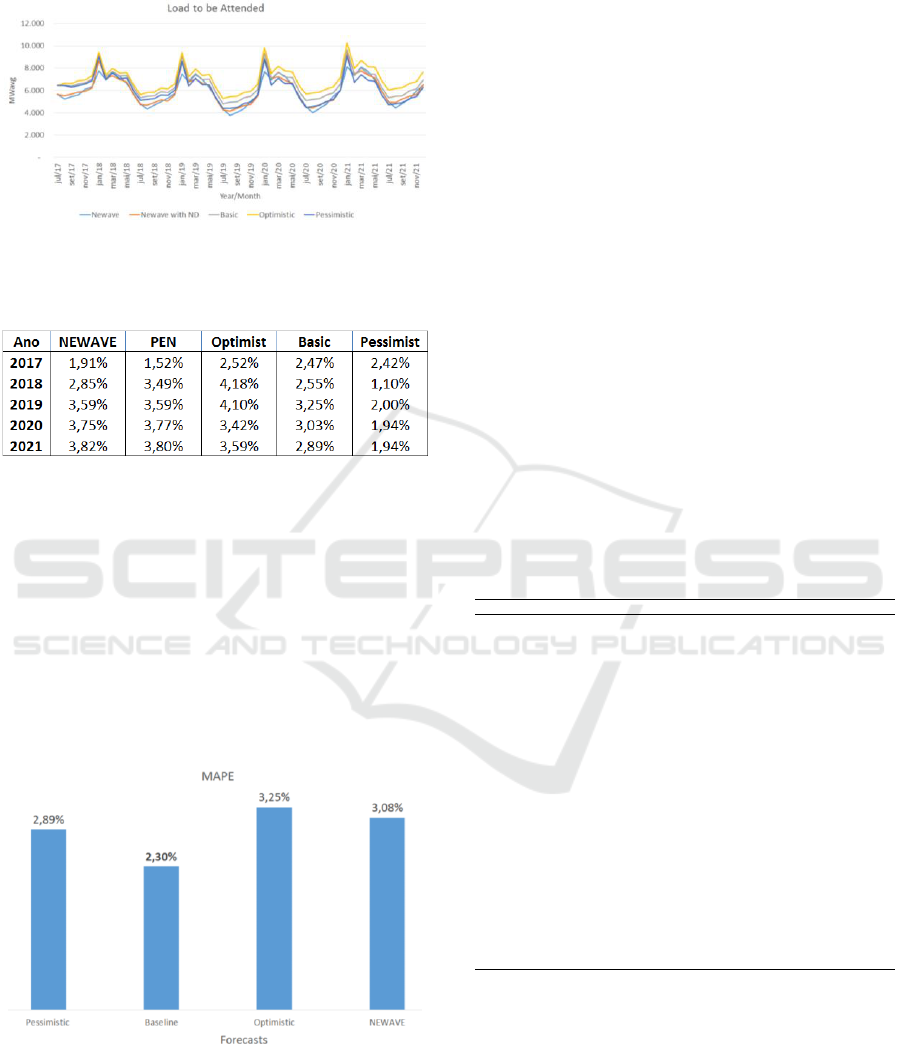
optimist than the ones presented on the baseline
scenario.
Figure 8: Load Forecasting: System Operator Forecast
versus Alternative Scenarios.
Table 1: Power Demand Growth Rates.
Figure 9 presents the forecasting accuracy analysis,
considering the System Operator official forecasts
and the three scenarios build in this article. This
analysis was made considering scenarios forecasts
conceived by the authors in the last four years (11
times in total) as well as official forecasts made
available by the system operator (NEWAVE).
It is possible to observe that, on average, the baseline
scenario (the scenario with the highest probability of
occurrence) presents the lowest MAPE followed by
the pessimistic scenario and then the System Operator
official forecasts (NEWAVE).
Figure 9: Load Forecasting - System Operator versus
Alternative Scenarios.
Through this analysis, it is possible to notice that the
baseline scenario obtained via ADL model perform
better than the official model. The next step in the
analysis is to use the demand load forecasts aligned
with the simulated wind power generation to get
estimations for energy storage and thermal generation
forecasts.
3.2 Wind Power Generation
This subsection applies the method described on
subsection 2.2.2 to simulate wind power generation
on the northeast subsystem for the period between
July/2017 and December/2021. The study uses 2016
as the base year, therefore all the daily wind speed
extracted from Climate Forecast System Reanalysis -
CFSR and hourly load curves (provided by the
Syatem Operator - ONS) comprehends the period
between 1
st
January and 31
st
December/2016. In
July/2017, according to the Regulatory Authority -
ANEEL, there were, in the northeast, 362 wind farms
operating, 144 wind farms being constructed and 127
authorized to be constructed. Therefore, in total 597
wind farms are considered in the analysis, using the
starting operation data to define its generation amount
per month.
To transform the monthly power load forecasts into
hourly power load forecasts the monthly load curves
presented on Table 2 were used.
Table 2: Hourly Load Profile per Month.
Figure 10 presents the wind power generation
obtained after executing all the steps presented on
subsection 2.2.2. The System Operator forecasts
(NEWAVE) and the wind generation simulated in
this article is shown on Figure 10 and it is possible to
observe that, on average, wind power generation
provided by the System Operator is higher than the
one simulated, especially on peaks and valleys.
Besides of that, both have the same trend and behavior
Jan
Fev
Mar
Abr
Mai
Jun
Jul
Ago
Set
Out
Nov
Dez
Hora 1
1.06
1.05
1.03
1.02
1.01
1.00
1.00
1.00
1.01
1.03
1.05
1.07
Hora 2
1.02
1.01
0.99
0.98
0.97
0.96
0.96
0.96
0.96
0.99
1.01
1.03
Hora 3
0.98
0.97
0.95
0.95
0.94
0.93
0.93
0.92
0.93
0.96
0.98
0.99
Hora 4
0.96
0.94
0.93
0.92
0.92
0.91
0.91
0.90
0.91
0.93
0.94
0.96
Hora 5
0.94
0.92
0.91
0.91
0.91
0.90
0.90
0.89
0.90
0.92
0.92
0.94
Hora 6
0.92
0.91
0.90
0.90
0.90
0.89
0.89
0.89
0.89
0.91
0.91
0.93
Hora 7
0.92
0.89
0.85
0.85
0.85
0.85
0.86
0.85
0.83
0.86
0.89
0.91
Hora 8
0.85
0.85
0.84
0.85
0.85
0.85
0.86
0.86
0.85
0.84
0.83
0.84
Hora 9
0.86
0.87
0.92
0.93
0.93
0.93
0.93
0.93
0.94
0.89
0.85
0.86
Hora 10
0.93
0.95
1.00
1.00
1.00
1.01
1.00
1.01
1.01
0.97
0.93
0.93
Hora 11
1.00
1.01
1.03
1.03
1.03
1.04
1.03
1.04
1.04
1.02
1.01
1.00
Hora 12
1.03
1.03
1.05
1.05
1.05
1.06
1.05
1.06
1.06
1.05
1.04
1.03
Hora 13
1.05
1.05
1.05
1.04
1.05
1.05
1.05
1.05
1.05
1.05
1.06
1.05
Hora 14
1.04
1.04
1.03
1.03
1.03
1.03
1.03
1.03
1.04
1.04
1.05
1.04
Hora 15
1.02
1.04
1.07
1.06
1.06
1.06
1.05
1.07
1.07
1.05
1.03
1.03
Hora 16
1.05
1.07
1.08
1.07
1.07
1.07
1.06
1.08
1.08
1.07
1.07
1.06
Hora 17
1.06
1.07
1.06
1.05
1.05
1.06
1.05
1.06
1.06
1.06
1.08
1.07
Hora 18
1.04
1.04
1.01
1.01
1.02
1.02
1.02
1.03
1.02
1.04
1.06
1.04
Hora 19
1.00
0.99
0.97
1.04
1.07
1.07
1.06
1.04
1.05
1.04
1.02
1.00
Hora 20
0.96
0.98
1.06
1.07
1.08
1.08
1.10
1.09
1.08
1.06
1.02
0.97
Hora 21
1.08
1.06
1.04
1.05
1.05
1.05
1.06
1.06
1.05
1.06
1.07
1.06
Hora 22
1.07
1.06
1.05
1.05
1.05
1.04
1.05
1.05
1.04
1.05
1.05
1.05
Hora 23
1.06
1.07
1.09
1.09
1.08
1.08
1.08
1.08
1.08
1.06
1.05
1.04
Hora 24
1.09
1.09
1.07
1.06
1.05
1.05
1.05
1.05
1.05
1.06
1.08
1.08
Improvements in the Current Brazil’s Energy Dispatch Optimization: Load Forecast and Wind Power
403
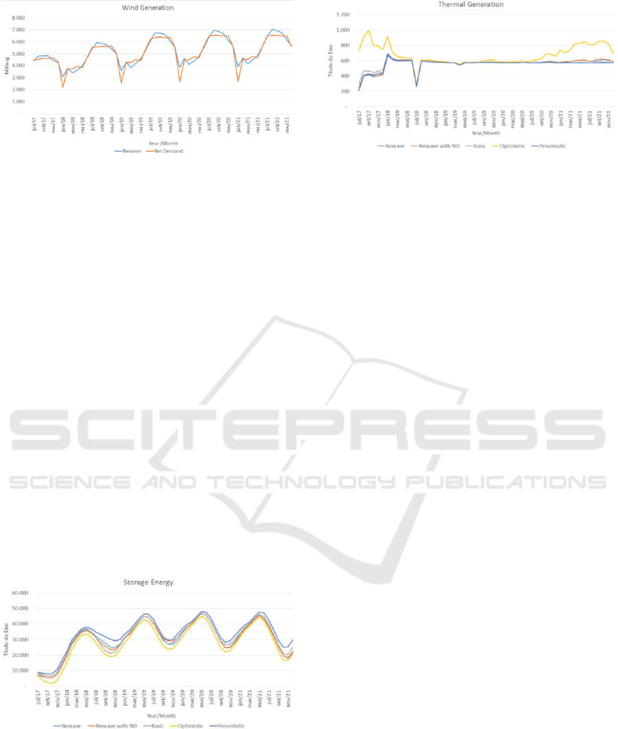
Figure 10: Wind Generation: System Operator versus
Simulation.
The load to be attended (Figure 7) is higher on the
basic scenario than on the System Operator Forecast
(with wind power simulation abatement) and on
System Operator Forecasts itself. The optimist
scenario is the one with the highest load to be
attended.
Considering the data from the load to be attended in
all scenarios (Figure 7), it is possible to evaluate,
using the hydrothermal dispatch model, which would
be the system behavior according with the power
demand forecasts and wind power generation
simulated.
Figure 11 presents the Storage Energy and Figure 12
contains the Thermal Generation for each scenario
conceived. From Figure 11 it is possible to notice that
the energy stored considering the System Operator
Forecasts is higher than the basic scenario and the
optimist scenario, but lower than the pessimist
scenario. Comparing the System Operator Forecasts
(with wind power simulation abatement) and the
System Operator Forecasts itself, it is possible to
notice that the energy stored in this case is lower than
in the traditional model.
Figure 11: Energy Storage.
For the thermal generation, only the optimist scenario
demands higher thermal generation. On average, the
baseline scenario demands a little bit less thermal
generation than the NEWAVE scenarios.
Figure 12: Thermal Generation.
4 CONCLUSIONS
The study contains a nouvelle approach to introduce
wind power generation on the Brazilian Dispatch
model, using MCMC to simulate wind power
generation instead of using the traditional historical
monthly wind power generation. Additionally,
additive distributed lags - ADL models were
conceived to estimate power demand forecast per
month, by subsystem. All the analysis in the article
was done applying both approaches in the Brazilian
northeast subsystem, considering de forecast period
between July/2017 and December/2021. Concerning
the power demand forecasts, one can notice that the
baseline scenario provide more accurate forecasts
than the System Operator forecasts, which has
accuracy lower than the pessimist scenario. Changing
the power demand forecasts for more accurate
approaches would provide better price signals and
dispatch signalizations to the system operator.
The introduction of wind power generation using
stochastic simulation and therefore a new approach to
estimate the net demand, showed little impact on the
thermal energy generation, but generated
considerable differences when it comes to the load to
be attended and energy storage. For the future, the
idea is to introduce probabilistic demand forecasts on
the dispatch model and to make further improvements
on the way wind power and solar energy would be
considered on the dispatch model.
ACKNOWLEDGEMENTS
This study was financed in part by the Coordenação
de Aperfeiçoamento de Pessoal de Nível Superior -
Brasil (CAPES) - Finance Code 001. The authors also
thank the R and D program of the Brazilian Electricity
Regulatory Agency (ANEEL) for the financial
support (P and D 0387-0315/2015) and the support of
the National Council of Technological and Scientific
ICORES 2019 - 8th International Conference on Operations Research and Enterprise Systems
404

Development (CNPq - 304843/2016-4) and FAPERJ
(202.673/2018).
REFERENCES
OTexts, “Forecasting: Principles and Practice, Advanced
Forecasting Methods, Dynamic Regression”. Acessed:
October 2018. https://otexts.org/fpp2/dynamic.html
Almutairi, A; Hassan Ahmed, M.; Salama, M. M. A., 2016.
“ Use of MCMC to incorporate a wind power model for
the evaluation of generating capacity adequacy”.
Electric Power Systems Research, v. 133, p. 63–70,
2016.
Alexiadis, M. C. et al. Short-term forecasting os Wind
speed and related electrical power. Solar Energy, v. 83,
p. 61–68, 1998.
Almutairi, A.; Hassan Ahmed, M.; Salama, M. M. A. Use
of MCMC to incorporate a wind power model for the
evaluation of generating capacity adequacy. Electric
Power Systems Research, v. 133, p. 63–70, 2016.
Aneel. Big - Banco de Informações de Geração [Generation
Information Bank]. Available in:
<http://www2.aneel.gov.br/aplicacoes/capacidadebrasi
l/capacidadebrasil.cfm>. Access in: 5 nov. 2017.
Billinton, R.; Chen, H.; Ghajar, R. Time-series models for
reliability evaluation of power systems including wind
energy. Microeletronic Reliability, v. 36, n. 9, p. 1253–
1261, 1996.
Castino, F.; Festa, R.; Ratto, C. F. Stochastic modelling of
Wind velocities time series. Journal of Wind
Engineering and Industrial Aerodynamics, v. 74–76, p.
141–151, 1998.
CCEE. Virtual Library. Available in:
<https://www.ccee.org.br/portal/faces/acesso_rapido_
header_publico_nao_logado/biblioteca_virtual?palavra
chave=Conjunto de arquivos para
cálculo&_afrLoop=870851647413887&_adf.ctrl-
state=9ll9uhpyu_27#!%40%40%3F_afrLoop%3D870
851647413887%26palavrachave%3DConjunto%2Bde
%2Barquivos%2Bpara%2Bc%25C3%25A1lculo%26_
adf.ctrl-state%3D9ll9uhpyu_31>. Access in: 8 dec.
2017.
Iversen, E. et al. Short-term probabilistic forecasting of
wind speed using stochastic differential equations.
International Journal of Forecasting, v. 32, n. 3, p. 981–
990, 2016.
Jung, J.; Broadwater, R. Current status and future advances
for Wind speed and power forecasting. Renewable and
Sustainable Energy Reviews, v. 31, p. 762–777, 2014.
Landry, M. et al. Probabilistic gradient boosting machines
for GEFCom2014 wind forecasting. International
Journal of Forecasting, v. 32, n. 3, p. 1061–1066, 2016.
Leite Da Silva, A. M.; Melo, A. C. G.; Cunha, S. H. F.
Frequency and duration method for reliability
evaluation of large-scale hydrothermal generating
systems. Generation Transmission and Distribution,
IEE Proceedings C, v. 138, n. 1, p. 94–102, 1991.
Manwell, J. F.; Mcgowan, J. G.; Rogers, A. L. Wind Energy
Explained: Theory, Design and Application. [s.l: s.n.].
Oliveira, F. L. C.; Souza, R. C.; Marcato, A. L. M. A time
series model for building scenarios trees applied to
stochastic optimisation. International Journal of
Electrical Power and Energy Systems, v. 67, p. 315–
323, 2015.
ONS. Histórico da Operação - Geração de Energia
Available: <http://www.ons.org.br/Paginas/resultados-
da-operacao/historico-da-
operacao/geracao_energia.aspxx>
Papaefthymiou, G.; Klöckl, B. MCMC for wind power
simulation. IEEE Transactions on Energy Conversion,
v. 23, n. 1, p. 234–240, 2008.
Pinson, P. Wind energy: forecasting challenges for its
operational management. Statistical Science, v. 28, n. 4,
p. 564–585, 2013.
Saha, S. et al. NCEP Climate Forecast System Version 2
(CFSv2) Selected Hourly Time-Series Products.
Available: <https://doi.org/10.5065/D6N877VB>.
Access in: 3 mar. 2017.
Suomalainen, K. et al. Correlation analysis on wind and
hydro resources with electricity demand and prices in
New Zealand. Applied Energy, v. 137, p. 445–462,
2015.
Zhang, Y.; Wang, J.; Wang, X. Review on probabilistic
forecasting of wind power generation. Renewable and
Sustainable Energy Reviews2, v. 32, p. 255–270, 2014.
Improvements in the Current Brazil’s Energy Dispatch Optimization: Load Forecast and Wind Power
405
