A Simulation-based Optimisation Approach

for Inventory Management of Highly Perishable Food

Ning Xue

, Dario Landa-Silva

, Grazziela P. Figueredo

and Isaac Triguero

ASAP Research Group, School of Computer Science, University of Nottingham, U.K.

IMA Research Group, School of Computer Science, University of Nottingham, U.K.

Keywords:

Highly Perishable Food Inventory, Discrete Event Simulation, Particle Swarm Optimisation.

Abstract:

The taste and freshness of perishable foods decrease dramatically with time. Effective inventory management

requires understanding of market demand as well as balancing customers needs and preferences with prod-

ucts’ shelf life. The objective is to avoid food overproduction as this leads to waste and value loss. In addition,

product depletion has to be minimised, as it can result in customers reneging. This study tackles the produc-

tion planning of highly perishable foods (such as freshly prepared dishes, sandwiches and desserts with shelf

life varying from 6 to 12 hours), in an environment with highly variable customers demand. In the scenario

considered here, the planning horizon is longer than the products’ shelf life. Therefore, food needs to be re-

plenished several times at different intervals. Furthermore, customers demand varies signiﬁcantly during the

planning period. We tackle the problem by combining discrete-event simulation and particle swarm optimisa-

tion (PSO). The simulation model focuses on the behaviour of the system as parameters (i.e. replenishment

time and quantity) change. PSO is employed to determine the best combination of parameter values for the

simulations. The effectiveness of the proposed approach is applied to some real-world scenario correspond-

ing to a local food shop. Experimental results show that the proposed methodology combining discrete event

simulation and particle swarm optimisation is effective for inventory management of highly perishable foods

with variable customers demand.

1 INTRODUCTION

Effective planning is important in production systems

that aim at effective management and coordination

of related activities and resources for an organisation

(Makui et al., 2016). A common aim in such sys-

tems is to achieve optimal production planning and

inventory management to meet (often variable) prod-

ucts demand over the planning horizon (Ramezanian

et al., 2012). Within the food production sector, pro-

ducers aim at delivering optimal planning to manage

supply/demand effectively. Perishability is a key at-

tribute that cannot be ignored in food supply chain

management. Critical decisions must be made regard-

ing the replenishment of food items in the right time

and quantity with the goal of maximising proﬁt while

minimising complete stock depletion and waste.

This paper tackles inventory management of

highly perishable food with a very limited shelf life

and with variable customers demand. We focus on a

scenario in the hospitality sector, that of shops selling

foods such as freshly prepared dishes, sandwiches and

desserts. The production planning period is longer

than the shelf life of the products. This means that

products need to be replenished frequently during

the planning period. In addition, customers demand

for the foods varies greatly over time. A particular

strain is put into production, when rare and/or extreme

external events occur. For instance, when demand

changes dramatically due to weather conditions, spe-

cial events (e.g. holiday season, football matches) and

promotions. Production planning and inventory man-

agement under such conditions is difﬁcult and subject

to high uncertainty.

Planning problems involving such complexity of-

ten require the use of simulation models to understand

the behaviour of the system as parameters change.

The abstracted simulation model is capable of encom-

passing the stochasticity and the variabitity found in

the real-world, therefore assisting in addressing the

problem’s complexity. Also, detailed reports regard-

ing the dynamic of the system and the simulation out-

puts can be extracted for further analysis and to be

employed as inputs to future optimisation exercises

406

Xue, N., Landa-Silva, D., Figueredo, G. and Triguero, I.

A Simulation-based Optimisation Approach for Inventory Management of Highly Perishable Food.

DOI: 10.5220/0007401304060413

In Proceedings of the 8th International Conference on Operations Research and Enterprise Systems (ICORES 2019), pages 406-413

ISBN: 978-989-758-352-0

(Duong and Wood, 2018). We apply discrete event

simulation (DES) to understand the behaviour of the

system as parameters (i.e. replenishment time and

quantity) change. Discrete events at particular times

such as sales and food expiring are simulated as the

changes of state in the system. A Particle Swarm Op-

timisation (PSO) algorithm (Shi and Eberhart, 1998)

is implemented to determine the best combination of

parameter values that leads to an optimal solution.

We investigate the optimisation of replenishment time

and quantities in the tackled scenario. Experimental

results using real-world data from a food shop demon-

strate the effectiveness of the proposed method for

tackling inventory management of highly perishable

foods with variable customers demand.

Problems related to the planning of perishable in-

ventories and ordering policies arise in different sec-

tors including food, chemicals, drugs and blood banks

(Vila-Parrish et al., 2008). Regarding modelling tech-

niques and mathematical methods, linear program-

ming, integer or mixed integer programming are the

most dominant methods, please refer to (Soto-Silva

et al., 2016) for model details. Literature reviews on

perishable inventory systems can be found in (Fergu-

son et al., 2007), (Bakker et al., 2012), (Yu et al.,

2012) ,(Bushuev et al., 2015). Perishable inventory

research to date has made a lot of progress on food

sectors of grocery retailers context, where the shelf

life usually ranges from several days to months. To

the best of our knowledge, this is the ﬁrst attempt to

address the problem of inventory planning of perish-

able food with shelf life of just a few hours.

The remainder of this paper is organised as fol-

lows: the problem is described in detail in Section

2; the solution method is presented in Section 3; the

computational experiments follow in Section 4; ﬁ-

nally conclusions are drawn in the last section.

2 PROBLEM DESCRIPTION

We model the food production of a food shop that

produces and sells fresh prepared dishes, sandwiches

and desserts. The shop usually opens at 7:00AM sell-

ing items produced early that morning and leftover

items produced the night before. It is expected that

the number of leftover items from the night before is

enough to cover demand until around 10:00AM. Af-

ter that, food items produced after the shop opens are

served to customers. Depending on the demand, prod-

uct shelves will be replenished several times in a day.

To aim for freshness, food items are marked as ex-

pired after 6 to 12 hours (exact time depends on the

product type) on the shelf. The expired product is

subsequently thrown away. If food items are prepared

and placed in the shelves too early and not sold out be-

fore they have perished then waste may occur. How-

ever, items not prepared on time to supply demand

may result in customers reneging (i.e. customers leav-

ing because the preferred item is out of stock). Due

to this dynamic complexity, the store manager faces a

challenging problem of both preparing enough items

and reducing waste. The goal is to determine the re-

plenishment time and replenishment quantity for each

item that needs to be prepared in advance, in order to

minimise food wastage and running out of inventory

(i.e., ‘a stock out’).

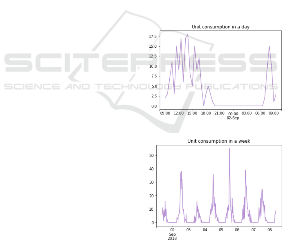
The items demand may change dramatically in a

day or week as shown in Figures 1 and 2, respectively.

In this paper we only predict the next day hourly de-

mand. Prediction beyond that is out of the scope of

this paper because of the sensitivity to the effect of

store promotions, weather, trafﬁc conditions and spe-

cial events (e.g. holiday, football match) which is not

yet considered here.

Figure 1: Demand ﬂuctuates considerably in a day.

Figure 2: Demand ﬂuctuates considerably in a week.

A Simulation-based Optimisation Approach for Inventory Management of Highly Perishable Food

407

2.1 Discrete Event Simulation Model

The following notation is used in the DES model:

• e: the number of items expiring.

• r: the number of customers reneging.

• w

: the weight of e in the objective function .

• w

: the weight of r in the objective function .

• t

: the ith replenishment time, t

< t

i+1

and t

∈ T .

• q

: the replenishment quantity at t

, q

∈ Q.

• (t

): the lower bound and the upper bound of t

respectively, in minutes.

• (q

, q

): the lower bound and the upper bound of

respectively, in units.

• l: the shelf life of an item, in minutes.

• (r

, r

): the lower bound and the upper bound for

calculating (t

), in minutes.

A solution to the inventory manage-

ment problem is encoded by two n-tuples

s =

{

, ..., t

}

{

, q

, ..., q

}

, representing

replenishment times and replenishment quantities,

respectively.

The problem can be formally deﬁned as follows:

minw

e + w

r (1)

subject to

≤ t

∀i ∈ I (2)

≤ q

∀i ∈ I (3)

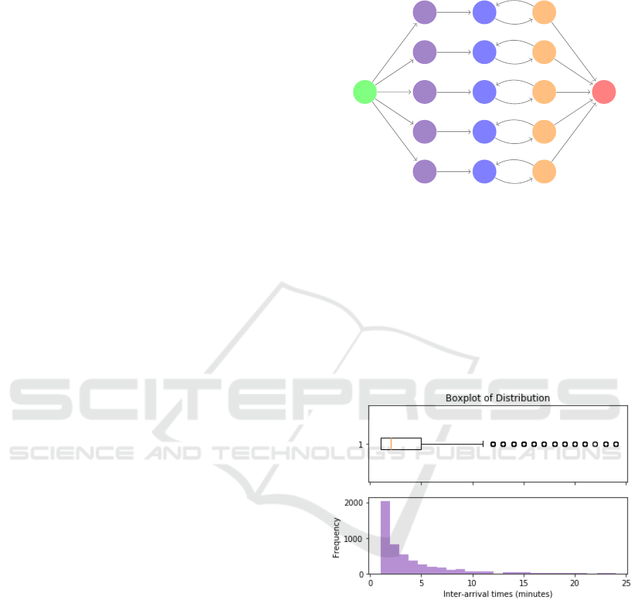
3 SOLUTION METHOD

We use the solution framework illustrated in Figure

3 to explore optimal replenishment time and quantity

for each item. The framework has 2 phases: 1) gener-

ate data for the simulation and 2) execute simulation-

based optimisation. The ﬁrst phase for generating

data, denoted DG, generates a set of traces for the

simulation according to predicted demand. For this, 5

replications are performed in this work, hence gener-

ating 5 traces. The aim of performing multiple repli-

cations is to produce multiple samples in order to ob-

tain a better estimate of mean performance. The sec-

ond phase, applies discrete event simulation to simu-

late each generated trace and the best combination of

parameters values (i.e. replenishment time and quan-

tity) for the simulation is determined by the PSO.

Demand

DES PSO

Output

Figure 3: Solution framework. The ﬁrst layer (green circle)

represents the demand; the second layer is the data genera-

tion, followed by the discrete event simulation phase (DES)

coupled with the particle swarm optimisation (PSO).

3.1 Data Generation

We generate trace data based on predicted hourly

sales. Each trace contains transaction time and the

number of units sold at that time. We ﬁrst analyse his-

torical customer arrival intervals for an item within a

recent month, as an example shown in Figure 4.

Figure 4: Frequency of customer arrival intervals for a given

item in a recent month.

The upper part of the graph shows the distribution

box plot. In the lower part, the horizontal axis shows

the interval in minutes of customer arrivals while the

vertical axis shows the frequency. The ﬁgure shows

that the inter-arrival times distribution is right skewed

with fat tails (with mean=3.67, median=2). In fact,

the shape of the distribution is similar to an expo-

nential distribution, namely Erlang distribution when

K = 1. Further exploration suggested that Erlang dis-

tribution (mean=3.67, and K=0.85) ﬁts well with the

historical data. We use a QQ (quantile quantile) plot

of inter-arrival distribution with the Erlang distribu-

ICORES 2019 - 8th International Conference on Operations Research and Enterprise Systems

408

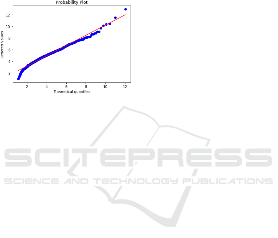
tion to do a more thorough check for the distribution.

It can be seen that most dots ﬁt the line, suggesting the

shape of the data matches the shape of the probability

density function of Erlang.

Figure 5: QQ (quantile quantile) plot of historical data and

simulated Erlang data.

Next, we generate the number of units that would

be sold in each transaction. This number is ran-

domly drawn with some probability from historical

data. Note that not all numbers are randomly gener-

ated as we have to ensure the total units in each hour

matches predicted values. Therefore, it is necessary to

ﬁx some values instead of generating them randomly.

3.2 Simulation-based Optimisation

At this stage, DES is applied to simulate each gener-

ated trace (Section 3.1). For each simulation with cer-

tain parameters values (i.e. replenishment time and

quantity), we calculate the objective function value

(Section 2.1), which is the solution ﬁtness in the PSO,

and update parameters values. Finding the best com-

bination of parameters values (i.e. replenishment time

and quantity) for the simulation is guided by the PSO.

The reason to use simulation to obtain the solution

ﬁtness is twofold: ﬁrstly, simulation can generate ran-

dom samples; secondly, due to the stochastic and dy-

namic complexity nature, the objective function is not

easy to be mathematically expressed and computed

directly.

3.2.1 Discrete Event Simulation

DES has been widely applied in production planning

due to its capability for modelling uncertainties that

lie in a planning process. A DES models the operation

of a system as a discrete sequence of events in time.

Each event, such as a customer consuming a product,

occurs at a particular time and changes the state of the

system. In the context of inventory management, the

optimisation procedure can be used to ﬁnd the most

suitable parameters for the simulation in order to ﬁnd

the best possible solutions to a problem. Optimisa-

tion techniques that have been applied to inventory

management can be widely classiﬁed into mathemat-

ical programming (e.g. linear/non-linear program-

ming) and direct search methods (e.g. gradient based,

statistical models, (meta)-heuristics). Please refer to

the review papers by (Arisha and Abo-Hamad, 2010)

(De Meyer et al., 2014) for more details.

3.2.2 Particle Swarm Optimisation

We implemented PSO to determine the best combi-

nation of parameters values for the simulation model

(Section 2.1. The reasons to adopt PSO as optimiser

for this problem are threefold: PSO is simple in im-

plementation; PSO uses simple fast to execute mathe-

matical operators and is efﬁcient in memory require-

ment, both essential for simulation based optimisa-

tion; and PSO is a general parameter value optimisa-

tion method which requires no assumptions about the

problem being optimised.

PSO is a population-based meta-heuristic intro-

duced by Eberhart and Kennedy (Kennedy, 1995)

that has been successfully applied to several inven-

tory management applications (Tsai and Yeh, 2008)

(Xu et al., 2013) (Park and Kyung, 2014). PSO is in-

spired on the social behaviour patterns of a biological

group such as a ﬂock of birds or a school of ﬁsh. In

the PSO method, a decision variable is regarded as

a particle, and the population of decision variables is

considered as a swarm. PSO was initially proposed

for continuous function optimisation. In this work

we truncate continuous values to integers when im-

plementing PSO as the number of units and time are

both expressed by integer values. Our experiments

here indicate that this truncation does not affect sig-

niﬁcantly the performance of the method, as it was

also found in other works (Laskari et al., 2002).

PSO is initialised with a group of random parti-

cles (solutions) and then the algorithm searches for

optima by updating generations of particles. In each

iteration of PSO, each particle is updated within its

given bounds by following two “best” values. The

ﬁrst one is the best solution that the particle and its

neighbours have achieved so far (local best). The

other one is the best solution found so far by any par-

ticle in the whole population (global best). Based on

these two best values, a particle updates its velocity

and positions. More details of how PSO works can

be found in (Kennedy, 1995) and (Shi and Eberhart,

1998). There are many variants (Rini et al., 2011) of

PSO, but in this paper we implemented the standard

A Simulation-based Optimisation Approach for Inventory Management of Highly Perishable Food

409

one (Kennedy, 1995). The ﬁtness of a particle is com-

puted by means of the simulation as mentioned pre-

viously, hence the approach being a simulation-based

optimisation technique.

4 EXPERIMENTS

The proposed solution method was implemented in

Python and run on a PC with Intel i7 2.40GHZ pro-

cessor and 4GB RAM, similar computing equipment

available in a typical food shop in the scenario con-

sidered here.

4.1 Problem Instance Data

A set of problem instances reﬂecting characteristics of

the real-world scenarios considered was generated by

a prediction model. Each instance contains predicted

hourly sales of an item in a day. Five instances of each

item are generated. The instances groups are called I6

and I12, where the number corresponds to shelf life.

For example, I6 are the instances where the shelf life

of the item is 6 hours.

4.2 Parameters Tuning

Considering the two objectives of minimising waste

and minimising the number of customers reneging,

we can think of trade-off solutions exhibiting a com-

promise between these two objectives. This is be-

cause arguably minimising waste (producing less)

could be in conﬂict with minimising reneging (pro-

ducing more). However, the desirable overall optimal

solution for our case will obviously have zero waste

and zero customers reneging.

Since the desired optimal solution will have 0

as the value for waste and customers reneging, the

goal is to ﬁnd the parameter values that quick-

est converge to 0 in the objective function. The

Irace package (L

opez-Ib

anez et al., 2011) is ap-

plied for parameter tuning using 4 selected instances

(I6 1, I6 2, I12 1, I12 2).

A standard implementation of the PSO algorithm

requires 4 parameters:

• Swarm size (n): Number of particles in the popu-

lation.

• Inertia (ω): Inertia weight in a particle’s move-

ment.

• Personal best attraction (phi

): Weight for parti-

cle’s pull towards its own best solution achieved

so far.

• Neighbour best attraction (phi

): Weight for pull

towards the global best solution.

The parameters, their range considered in the tun-

ing (based on some preliminary runs) and the best val-

ues found are given in Table 1. The maximum number

of experiments is set to 1000 and other parameters for

Irace are set to default values.

Table 1: Parameter Tuning for the PSO Using Irace.

Parameters Type Range Best

n C (5, 10, 20, 50

30, 40, 50,

60, 70, 80,

90, 100, 120,

140, 160, 180,

200, 240, 280,

, 320)

ω R (-2, 2) 0.637

phi

C (-4, -3.5, -3, 0.5

-2.5, -2, -1.5,

-1, -0.5, 0,

0.5, 1, 1.5,

2, 2.5, 3,

3.5, 4)

phi

C (-4, -3.5, -3, 1.5

-2.5, -2, -1.5,

-1, -0.5, 0,

0.5, 1, 1.5,

2, 2.5, 3,

3.5, 4)

C: Categorical

R: Real

4.3 Algorithm Performance

In order to analyse the performance of the proposed

solution method, we test the algorithm on 10 prob-

lem instances using the best-suited parameter values

given in Table 1. In order to obtain statistically sound

results, all experiments are conducted with 10 inde-

pendent runs (mean values were recorded) over all

10 problem instances. To obtain a better estimate of

mean performance, each experiment run is based on

the mean values of 5 simulations. Each simulation

is terminated after reaching an optimal solution (i.e.

with objective function value equal to 0 representing

the best ﬁtness). For each instance, all 10 runs start

with the same initial solution created at random.

The computation time for each problem instance

is given in Table 2. It can be seen that all instances

were solved well under 2 minutes. Solving the group

ICORES 2019 - 8th International Conference on Operations Research and Enterprise Systems

410

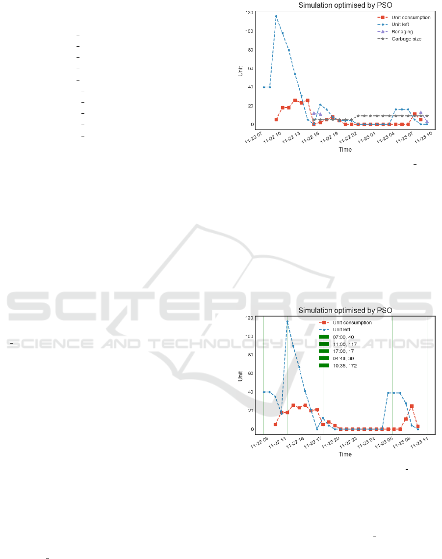
Table 2: Computation Times.

Instance Time(s)

I6 1 92.4

I6 2 81.6

I6 3 70.8

I6 4 60

I6 5 65

I12 1 31.2

I12 2 42

I12 3 34.8

I12 4 49.2

I12 5 34

of instances I6 requires more decision variables (be-

cause of more frequent replenishment), hence taking

longer computation time compared to instances I12.

We now describe some examples of replenishing

plans. Figure 6), is an example of such plan for an

instance with 6 hours shelf life. The horizontal axis

shows the length of the planning period (i.e. 1 day),

while the vertical axis shows the number of units of

an item. The Unit consumption line corresponds to

the total number of units sold during the day. The

Unit left line corresponds to the units available on the

shelf. The Reneging line is for the number of cus-

tomers reneging at different times during the day. The

Garbage size line is the cumulative sum of items that

have been thrown away due to expiration.

Figure 6 shows a non-optimal solution for instance

I6 1 found during the algorithm execution and before

reaching an optimal solution. This ﬁgure captures the

simulation scenario in which a large number of items

were replenished (unit left line) at around 10 am. This

large replenishment was sufﬁcient to cover the high

demand (unit consumption line) from 11 am to around

3 pm. Due to the faltering demand from 3pm onward,

the number of units left is higher that the consumption

by 4pm. However, because of the 6 hours shelf life of

the item, those leftovers have to be thrown away at

4pm. Since there was no fresh items produced and

placed timely on the shelf at 4pm, some customers

left because the item they wanted was out of stock.

A similar situation occurred later at night. It can be

seen that this is a non-optimal solution or inventory

management plan because the replenishment time and

quantity have led to both item wastage and customer

reneging.

Figure 7 shows an optimal solution for the same

instance I6 1 discussed above, in which there is no

item wastage and no customers reneging. The re-

plenishment times are represented by the vertical bars

and the corresponding replenishment time and quan-

tity are given in the legend. In this optimal solution,

it can be seen that although the unit left line is well

Figure 6: Non-optimal solution for instance I6 1.

above the unit consumption line, there is no wastage

or reneging because replenishment has been done ef-

fectively to supply demand. A typical convergence

rate of one simulation (i.e. simulation based on 1

trace) of this solution is given in Figure 8. The hori-

zontal axis corresponds to number of iterations while

the vertical axis corresponds to ﬁtness values. It can

be seen in the ﬁgure that convergence is very fast in

the ﬁrst 250 iterations and it slows down after that. Fi-

nally, an optimal solution was found just before 600

iterations.

Figure 7: Optimal solution for instance I6 1.

Another example of a replenishment plan, this

time for an instance for an item with 12 hours shelf

life, is shown in Figure 9. This plan is a non-

optimal solution obtained before an optimal solution

was found for problem instance I12 1. Similar to the

previous example, this ﬁgure captures the simulation

of a scenario in which a large number of items are re-

plenished at around 10am. Items have not been sold

out by 10pm and hence they are thrown away after the

12 hours shelf life passes. A number of items were

produced around 11pm. Demand increased from 7am

in the next day and customers consumed all items by

A Simulation-based Optimisation Approach for Inventory Management of Highly Perishable Food

411

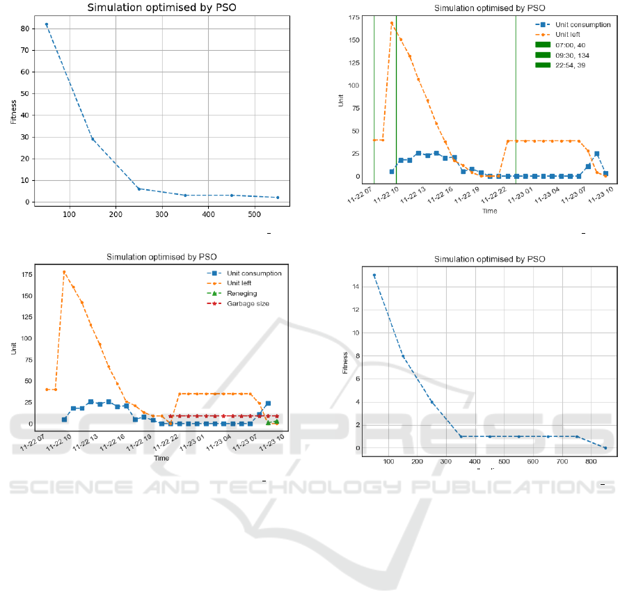
Figure 8: Convergence rate of solving instance I6 1.

Figure 9: Non-optimal solution for instance I12 1.

around 9am. As no replenishing takes place since

then, customers that arrived after 9am left after not

being able to supply their demand.

Figure 10 shows an optimal replenishment plan

with no item wastage or customers reneging. The

convergence rate of one simulation for this solution

is shown in Figure 11. This ﬁgure shows that conver-

gence is very fast within the ﬁrst 350 iterations and an

optimal solution is found before 900 iterations.

5 CONCLUSIONS

In this paper, we addressed an inventory management

problem considering a scenario in which food items

have very short shelf life and they need to be replen-

ished several times during the day in order to satisfy

demand, avoid wastage and avoid customers reneg-

ing. This problem arises in many restaurants and

other places in the hospitality sector. In the scenario

tackled here, the planning horizon is longer than the

shelf life of the food items. In addition, demand varies

considerably within the planning horizon. A replen-

Figure 10: Optimal solution for instance I12 1.

Figure 11: Convergence rate of solving instance I12 1.

ishment plan consists of determining the times dur-

ing the planning horizon in which food items should

be replenished and the corresponding quantities in or-

der to minimise waste and the number of customers

reneging.

We model this inventory problem using Discrete

Event Simulation (DES) to understand the dynam-

ics of the system as parameters change. Then, Par-

ticle Swarm Optimisation (PSO) is employed to de-

termine the best combination of parameter values for

the simulations. Experimental results on 10 prob-

lem instances have demonstrated the effectiveness of

the proposed simulation-based optimisation approach

for solving different problem instances. This solu-

tion framework could be easily adapted to other sim-

ilar inventory replenishment scenarios. For instance,

to minimise perishable wastage in restaurants, super-

markets and hospitals. Particular beneﬁt could also

be obtained when venues need to comply with more

strict regulations due to the nature of the clientele,

such as pregnant women, immunocompromised indi-

viduals, and transplant patients.

Although the solution quality and computation

ICORES 2019 - 8th International Conference on Operations Research and Enterprise Systems

412

time in this work are acceptable by the typical store

manager, the abstract model created for simulation

still does not yet reﬂect the entire complexity of the

shop production dynamics. Further work will be un-

dertaken to improve the current model to enable even

better decision support. One aspect to be considered

is the inclusion of the food preparation process and

defrosting times, rather than just focusing on deter-

mining replenishment times and quantity. Also, an in-

depth study comparing the PSO to other optimisation

methods could also be an interesting future research

direction.

ACKNOWLEDGEMENTS

This research was supported by and PXtech Limited

and Innovate UK.

REFERENCES

Arisha, A. and Abo-Hamad, W. (2010). Simulation optimi-

sation methods in supply chain applications: a review.

Bakker, M., Riezebos, J., and Teunter, R. H. (2012). Re-

view of inventory systems with deterioration since

2001. European Journal of Operational Research,

221(2):275–284.

Bushuev, M. A., Guiffrida, A., Jaber, M., and Khan, M.

(2015). A review of inventory lot sizing review papers.

Management Research Review, 38(3):283–298.

De Meyer, A., Cattrysse, D., Rasinm

aki, J., and Van Or-

shoven, J. (2014). Methods to optimise the design and

management of biomass-for-bioenergy supply chains:

A review. Renewable and sustainable energy reviews,

31:657–670.

Duong, L. N. K. and Wood, L. C. (2018). Discrete event

simulation in inventory management. In Encyclopedia

of Information Science and Technology, Fourth Edi-

tion, pages 5335–5344. IGI Global.

Ferguson, M., Jayaraman, V., and Souza, G. C. (2007).

Note: An application of the eoq model with nonlin-

ear holding cost to inventory management of perish-

ables. European Journal of Operational Research,

180(1):485–490.

Kennedy, R. (1995). J. and eberhart, particle swarm opti-

mization. In Proceedings of IEEE International Con-

ference on Neural Networks IV, pages, volume 1000.

Laskari, E. C., Parsopoulos, K. E., and Vrahatis, M. N.

(2002). Particle swarm optimization for integer pro-

gramming. In Evolutionary Computation, 2002.

CEC’02. Proceedings of the 2002 Congress on, vol-

ume 2, pages 1582–1587. IEEE.

opez-Ib

anez, M., Dubois-Lacoste, J., St

utzle, T., and

Birattari, M. (2011). The irace package, iterated

race for automatic algorithm conﬁguration. Tech-

nical report, Technical Report TR/IRIDIA/2011-004,

IRIDIA, Universit

e Libre de Bruxelles, Belgium.

Makui, A., Heydari, M., Aazami, A., and Dehghani, E.

(2016). Accelerating benders decomposition approach

for robust aggregate production planning of products

with a very limited expiration date. Computers & In-

dustrial Engineering, 100:34–51.

Park, K. and Kyung, G. (2014). Optimization of total in-

ventory cost and order ﬁll rate in a supply chain using

pso. The International Journal of Advanced Manufac-

turing Technology, 70(9-12):1533–1541.

Ramezanian, R., Rahmani, D., and Barzinpour, F. (2012).

An aggregate production planning model for two

phase production systems: Solving with genetic algo-

rithm and tabu search. Expert Systems with Applica-

tions, 39(1):1256–1263.

Rini, D. P., Shamsuddin, S. M., and Yuhaniz, S. S. (2011).

Particle swarm optimization: technique, system and

challenges. International journal of computer appli-

cations, 14(1):19–26.

Shi, Y. and Eberhart, R. (1998). A modiﬁed particle swarm

optimizer. In Evolutionary Computation Proceedings,

1998. IEEE World Congress on Computational Intel-

ligence., The 1998 IEEE International Conference on,

pages 69–73. IEEE.

Soto-Silva, W. E., Nadal-Roig, E., Gonz

alez-Araya, M. C.,

and Pla-Aragones, L. M. (2016). Operational research

models applied to the fresh fruit supply chain. Euro-

pean Journal of Operational Research, 251(2):345–

355.

Tsai, C.-Y. and Yeh, S.-W. (2008). A multiple objective par-

ticle swarm optimization approach for inventory clas-

siﬁcation. International journal of production Eco-

nomics, 114(2):656–666.

Vila-Parrish, A. R., Ivy, J. S., and King, R. E. (2008).

A simulation-based approach for inventory modeling

of perishable pharmaceuticals. In Simulation Con-

ference, 2008. WSC 2008. Winter, pages 1532–1538.

IEEE.

Xu, J., Zeng, Z., Han, B., and Lei, X. (2013). A dynamic

programming-based particle swarm optimization al-

gorithm for an inventory management problem under

uncertainty. Engineering Optimization, 45(7):851–

880.

Yu, Y., Wang, Z., and Liang, L. (2012). A vendor managed

inventory supply chain with deteriorating raw materi-

als and products. International Journal of Production

Economics, 136(2):266–274.

A Simulation-based Optimisation Approach for Inventory Management of Highly Perishable Food

413