Impact of Sensing Film’s Production Method on Classiﬁcation Accuracy

by Electronic Nose

Ana P

adua

, Jonas Gruber

, Hugo Gamboa

and Ana Cec

ılia Roque

UCIBIO, REQUIMTE, Departamento de Qu

ımica, Faculdade de Ci

encias e Tecnologia da Universidade NOVA de Lisboa,

2829-516 Caparica, Portugal

Departamento de Qu

ımica Fundamental, Instituto de Qu

ımica da Universidade de S

ao Paulo, Av. Prof. Lineu Prestes,

748 CEP 05508-000, S

ao Paulo, SP, Brazil

Laborat

orio de Instrumentac¸

ao Engenharia Biom

edica e F

ısica da Radiac¸

ao (LIBPhys-UNL), Departamento de F

ısica,

Faculdade de Ciencias e Tecnologia da Universidade NOVA de Lisboa, 2829-516 Caparica, Portugal

Keywords:

Electronic Nose, Volatile Organic Compounds, Spin Coating, Film Coating, Machine Learning.

Abstract:

The development of gas sensing materials is relevant in the ﬁeld of non-invasive biodevices. In this work, we

used an electronic nose (E-nose) developed by our research group, which possess versatile and unique sensing

materials. These are gels that can be spread over the substrate by Film Coating or Spin Coating. This study

aims to evaluate the inﬂuence of the sensing ﬁlm spreading method selected on the classiﬁcation capabilities of

the E-nose. The methodology followed consisted of performing an experiment where the E-nose was exposed

to 13 different pure volatile organic compounds. The sensor array had two sensing ﬁlms produced by Film

Coating, and other two produced by Spin Coating. After data collection, a set of features was extracted from

the original signal curves, and the best were selected by Recursive Feature Elimination. Then, the classiﬁcation

performance of Multinomial Logistic regression, Decision Tree, and Na

ıve Bayes was evaluated. The results

showed that both spreading methods for sensing ﬁlms production are adequate since the estimated error of

classiﬁcation was inferior to 4 % for all the classiﬁcation tools applied.

1 INTRODUCTION

An electronic nose is a device able to detect and iden-

tify odours. The way it works is inspired in the mam-

malian’s olfactory system (Sankaran et al., 2012), ha-

ving two main parts: the perception and the recogni-

tion. The perception instrument has a delivery system

(to carry the gas sample from the sample to the detec-

tor), a detection system with a sensor array (where the

interaction with the gas sample occurs), and a trans-

duction and data collection system (that converts the

properties changing in the sensors into electrical sig-

nals) (Peris and Escuder-Gilabert, 2009). And the re-

cognition part includes mathematical methods for fe-

atures extraction and selection, as well as algorithms

for pattern recognition (Yan et al., 2015).

The sensors might be based on Surface Acou-

stic Wave (SAW), Quartz Crystal Microbalance

(QCM), Conducting Polymers (CP), Metal Oxide Se-

miconductors (MOS), optical sensors, among others

(Guti

errez and Horrillo, 2014). Each sensor reacts to

the presence of the odour in a different way, depen-

ding on its own sensibility and speciﬁcity. The pat-

terns of odours generated, also called ”ﬁngerprint”,

are electrical signals that result from the variance of

the sensor properties, such as conductance, voltage

and capacity. Furthermore, the signals acquired are

analysed, the best features are scored, and a pattern

recognition method is applied. For instance, Princi-

pal Component Analysis (PCA) has been employed to

reduce the number of features extracted from the sig-

nals (Ghasemi-Varnamkhasti et al., 2015), (Ordukaya

and Karlik, 2017). Additionally, machine learning al-

gorithms are commonly used for odours recognition

(Phaisangittisagul et al., 2010), (Zhang et al., 2008),

and (Barbri et al., 2009) , and are also employed for

concentration prediction (Xu et al., 2016).

Machine learning algorithms are becoming very

important for medical data analysis. For instance,

Decision Tree is a transparent and easily interpreta-

ble method, presenting a high potential for diagnostic

model building. (Polaka et al., 2017).

We created a home-made E-nose based on optical

sensors, which possess a new class of sensing ma-

Pádua, A., Gruber, J., Gamboa, H. and Roque, A.

Impact of Sensing Film’s Production Method on Classiﬁcation Accuracy by Electronic Nose.

DOI: 10.5220/0007401900560064

In Proceedings of the 12th International Joint Conference on Biomedical Engineering Systems and Technologies (BIOSTEC 2019), pages 56-64

ISBN: 978-989-758-353-7

terials invented by our research group. These gels

are very versatile and have unique stimuli-responsive

properties, altering their optical conﬁguration while

interacting with volatile organic compounds (VOCs)

(Hussain et al., 2017). This paper uses the E-nose

system we developed, which was previously descri-

bed in (Padua et al., 2018), for identiﬁcation of 13

different pure VOCs. Two different spreading met-

hod techniques have been used to produce our sensing

ﬁlms: Film Coating and Spin Coating. In this study,

we aim to test if sensing ﬁlms produced by different

spreading techniques have distinct VOCs discrimina-

tion capabilities.

Moreover, we were also interested in applying dif-

ferent machine learning algorithms for VOCs classi-

ﬁcation.

Support Vector Machine (SVM) for E-noses with

MOS sensors array (Ghasemi-Varnamkhasti et al.,

2015); and Neural network and the Large Margin Ne-

arest Neighbours (LMNN) for E-noses using SAW

sensors array (Hotel et al., 2018) produced the best

classiﬁcation results. However, when discrimination

can be done with a simple method, the usage of

more complex approaches is not needed (Ghasemi-

Varnamkhasti et al., 2015).

(Ordukaya and Karlik, 2017) compared the per-

formances of different machine learning algorithms

for olive oil classiﬁcation by an E-nose (Cyranose

320®): Na

ıve Bayes, k-Nearest Neighbours (k-NN),

Linear Discriminant Analysis (LDA), Decision Tree,

Artiﬁcial Neural Network (ANN), and SVM using

two different approaches: using dimensional re-

duction and without data reduction. The best success

rate was found with Na

ıve Bayes classiﬁer after data

reduction from 32 inputs to 8 inputs based on PCA.

The work of (Cho and Kurup, 2011) showed that

decision tree models have excellent results for classi-

ﬁcation and provide easily interpretable tree structure

for E-nose data. The decision tree approach was re-

ported as a promising pattern recognition method with

accuracy rates above 97 % using several features ex-

tracted from signals acquired by an E-nose based on

MOS sensors. The training of the decision tree was

also faster compared to Multilayer Perceptron (MLP)

and fuzzy ARTMAP classiﬁers.

(Siavash et al., 2018) developed a research where

used E-noses based on MOS sensors (FOX 400, Al-

pha M.O.S, France) and Field-Asymmetric Ion Mo-

bility Spectrometry (FAIMS, Owlstone Lonestar) to

distinguish healthy from diabetic patients. High pre-

diction accuracy was achieved by combining PCA

with a sparse logistic regression and a Gaussian pro-

cess classiﬁer. Another study used Logistic regres-

sion to classify data collected by an E-nose to iden-

tify correctly bioﬁlm-producing versus non bioﬁlm-

producing bacteria species with accuracy ranging

from 72.2 % to 100 %, depending on the organism

and methodology. When the dataset is not com-

plex, simple methods might be better than complica-

ted techniques to discriminate between different clas-

ses (Ghasemi-Varnamkhasti et al., 2015).

We decided to test three simple machine lear-

ning algorithms, since other authors have reported

the capability of other E-noses to perform classiﬁca-

tion of samples in a fast and reliable way using those

methods (Ordukaya and Karlik, 2017) (Ghasemi-

Varnamkhasti et al., 2015). In case we were not able

to achieve good performance, we intended to apply

more advanced computational techniques to enhance

classiﬁcation accuracy.

Taking into account the results obtained in the

previous studies, our study was focused on the per-

formance of Logistic Regression, Decision Tree and

ıve Bayes as data classiﬁer methods. Finally, the

class discrimination capabilities of these classiﬁers

were compared.

2 MATERIALS AND METHODS

2.1 Data Collection

A schematic of the E-nose system used is represented

in Figure 1. The device is composed of three main

parts: the delivery system, the detection chamber and

the transduction system.

The delivery system has two pumps working al-

ternately: the exposure pump, which creates a gra-

dient of pressure that transfers the headspace from the

sample chamber to the detection chamber; and the re-

covery pump, that is responsible for purging the de-

tection chamber (in the recovery periods).

The detection chamber is where the interaction of

the VOCs with the array of sensors takes place. Here,

the optical sensors that compose the array change

their optical properties while interacting with VOCs,

and these changes are detected by Light Dependent

Resistors (LDRs) and converted into electrical sig-

nals.

Signals’ collection is ensured by the transduction

system. It is composed of a microcontroller (Arduino

Due), that converts the analogue signals into digital

signals, and an embedded system (Raspberry Pi 2 Mo-

del B), for signals collection. More details about the

device have been earlier reported (Padua et al., 2018).

Inside the detection chamber, six optical sensors

based on tunable sensing ﬁlms were used in the sensor

array - see Figure 2 a).

Impact of Sensing Film’s Production Method on Classiﬁcation Accuracy by Electronic Nose

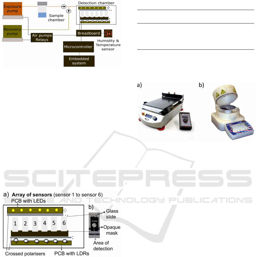
Figure 1: Schematic representation of E-nose V2.

Each sensor is composed of:

• a source of unpolarised light - a Light Emitting

Diode (LED);

• a sensing ﬁlm - based on tunable sensing gels des-

cribed in (Hussain et al., 2017) - sandwished bet-

ween two crossed polarising ﬁlters;

• a Light Dependent Resistor (LDR).

As shown in Figure 2 b), a sensing ﬁlm consists

of a thin layer of sensing gel spread on a glass slide

with a black mask on the back (that has a 5 mm di-

ameter hole, which delimiters the area of detection).

The sensing gels’ composition is based on a biopoly-

mer matrix with droplets of liquid crystal (LC), self-

assembled in the presence of ionic liquid (IL) (Hus-

sain et al., 2017).

Figure 2: a) Schematic of sensor array. ; b) Sensing ﬁlm.

In the present study, sensors nr 4 and 5 have sen-

sing ﬁlms produced by a standard (STD) recipe des-

cribed in Table 1, and sensors 1 and 3 are also pro-

duced by the standard recipe, plus adding 1.5 µL of

a cross-linking agent to the standard recipe, named

glutaraldehyde (GA), for 5 min at 500 RPM magnetic

stirring. Sensors 2 and 6 are controls: sensing ﬁlm 2

does not have IL and sensing ﬁlm 6 does not contain

LC.

After the gel’s production, the sensing ﬁlms might

be spread on the glass slides by two different ﬁlm

applicator equipment: Film Coater or Spin Coater.

The Film Coater used was the automatic ﬁlm appli-

cator with perforated heated vacuum bed from TQC

Table 1: Standard recipe for sensing ﬁlms production.

Component Time Magnetic Stirring

(min) (RPM)

BMIM DCA (IL) 10 300

5 CB (LC) 10 300

BSG 10-15 500

MilliQ water 5 500

IL = Ionic Liquid; LC = Liquid Crystal ; BSG = Bovine Skin Gelatin.

Sheen) - Figure 3 a), and the Spin Coater used was

the SPIN150i Tabletop from POLOS - Figure 3 b).

Figure 3: a) Film Coater ; b) Spin Coater.

The thickness of the sensing ﬁlms produced by

Film Coating is 30 µm, and the drop quantity of gel

used was 15 µL. Finally, the optical sensing ﬁlms with

light polarisation properties were obtained.

For this experiment, in the sensor array, sensing

ﬁlms 1 and 4 were spread by Film Coating (FC), whe-

reas sensing ﬁlms 3 and 5 were spread by Spin Coa-

ting (SC). A brief description of each sensor is provi-

ded in Table 2.

The experiment performed consisted in exposing

the same array of sensors (Table 2), placed inside the

detection chamber, to a set of 13 VOCs, sequentially,

in the following order: acetone, isopropanol, ethanol,

methanol, hexane, heptane, toluene, xylene, benzene,

chloroform, dichloromethane, diethyl ether, and ethyl

acetate. The experiment conditions are described in

the list below:

• VOC quantity: 20 mL

• Sample temperature: 37 °C

• Time exposure: 5 s

• Time recovery: 15 s

• Duration: 20 min

• Sampling rate: 5 Hz

The data was collected by the E-nose data trans-

duction and acquisition system. An example of a set

of 6 signals (one per sensor) acquired for exposure to

acetone is shown in Figure 4.

BIODEVICES 2019 - 12th International Conference on Biomedical Electronics and Devices

Table 2: Sensor array of the E-nose.

Sensor Sensing ﬁlm description Spreading technique

1 STD gel + GA FC

2 Control (without IL) FC

3 STD gel + GA SC

4 STD gel FC

5 STD gel SC

6 Control (without LC) SC

STD = Standard ; GA = Glutaraldehyde ; FC = Film Coating ; SC = Spin Coating ; LC = Liquid Crystal ; IL = Ionic Liquid.

2.2 Data Analysis

After data collection, the features related to each in-

dividual sensor were extracted. Table 3 describes the

8 features extracted per sensor, and Table 4 explains

the physicochemical meaning of each feature. Since

the sensor array is composed of 6 sensors, the num-

ber of original features that can be used is given by

6x8 = 48.

Then, auto-scaling was exploited for data pre-

processing, using a standardisation technique, accor-

ding to Eq. 1:

− ¯x

)

¯s

(1)

where Z

is the value of x

after auto-scaling. x

deﬁned as the variable before scaling. ¯x

is the varia-

ble mean and ¯s

is the standard deviation of the vari-

able. The ﬁnal value Z

varies around the mean zero

with standard deviation one.

2.2.1 Features Selection

We were interested in comparing the optical respon-

ses given by sensors where sensing ﬁlms that were

spread by Film Coating were applied, versus from

sensors with sensing ﬁlms that were spread by Spin

Coating.

Therefore, the original set of 48 features was di-

vided into two sub-groups (see Figure 5). One group

is composed by 16 features of sensing ﬁlms produ-

ced by Film Coating (sensors 1 and 4 - red signals in

Figure 4), and the other is composed by 16 features

of sensing ﬁlms produced by Spin Coating (sensors 3

and 5 - blue signals in Figure 4).

For each group of features, we were interested in

knowing the best number of features to select, and

what features were more interesting for VOCs classi-

ﬁcation.

Initially, each sub-group has 16 features. To

know the more relevant features for differentiating the

VOCs, Recursive Feature Elimination (RFE) was per-

formed. The estimator ’svc’ was used to assign weig-

hts to features. This estimator was trained on the ini-

tial set of features and the importance of each feature

was obtained. Then, the RFE method removes the

weakest features and selects them by recursively con-

sidering smaller and smaller sets of features. The pro-

cedure is recursively repeated on the pruned set until

a speciﬁc number of features to select is reached. For

each sub-group of features, RFE was used to select

the best number of features, and the top best were se-

lected by cross-validation (2 folds).

2.2.2 Classiﬁcation Models

We studied which classiﬁcation model works best for

sensors with sensing ﬁlms produced by Spin Coating

and Film Coating. To asses the quality of various pre-

diction methods, we trained models with three diffe-

rent classiﬁcation techniques: Multinominal Logistic

regression, Decision Tree, and Na

ıve Bayes.

Figure 6 shows the procedure used for each clas-

siﬁer. Each group of best features related to Film Co-

ating or Spin Coating was randomly divided in train

data (70 %) and test data (30 %).

Cross-validation (10 folds) was applied on the

train data. This means that the train set was rand-

omly divided in 10 subsets, using 9 for training the

model and the remaining to validate it. Firstly, the

model was built on the train set, then the training er-

ror was calculated; the validation set was tested se-

parately and the validation error was also obtained.

This procedure was repeated 9 more times, each time

using a different subset for validation. The average

over classes of cross-validation for the different clas-

siﬁcation techniques was reported. The parameters of

the models associated to a lower validation error were

selected for classiﬁers optimisation.

The parameters of optimisation were then applied

on the classiﬁer for prediction on the Test data. Fi-

nally, for each classiﬁer, the estimated error was cal-

culated, and the McNemar’s test was used to compare

the classiﬁers.

Impact of Sensing Film’s Production Method on Classiﬁcation Accuracy by Electronic Nose

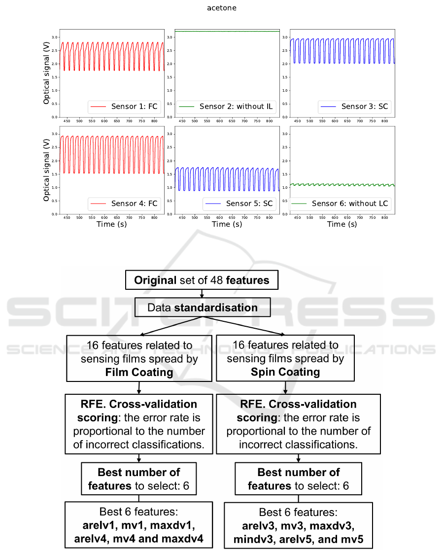
FC: sensor with sensing ﬁlm spread by Film Coating; SC: sensor with sensing ﬁlm spread by Spin Coating; IL: Ionic Liquid; LC: Liquid Crystal.

Figure 4: Examples of cycles from signals collected when the sensor array is cyclically exposed to acetone for 5 min, during

the 20 min experiment.

Figure 5: Schematic of features selection algorithm.

2.2.3 Na

ıve Bayes

ıve Bayes methods are a set of probabilistic algo-

rithms based on applying Bayes theorem with strong

independence assumption between every pair of fea-

tures.

For this work, we assumed the likelihood of the

features to be Gaussian. We applied the GaussianNB

BIODEVICES 2019 - 12th International Conference on Biomedical Electronics and Devices

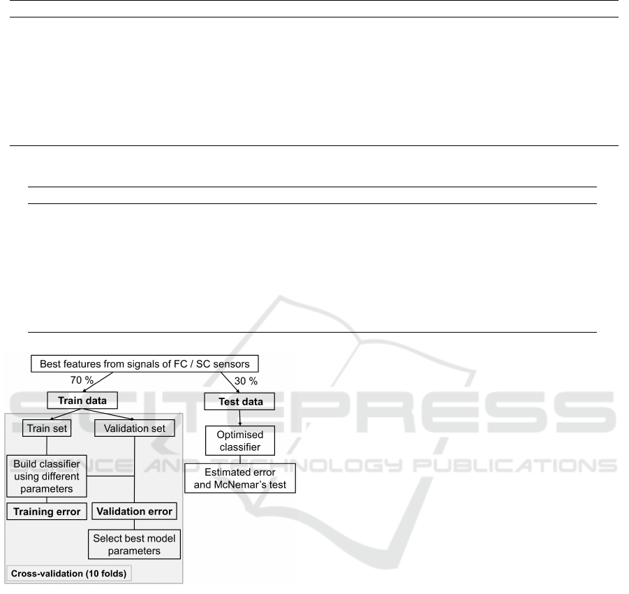
Table 3: Features extracted from the signals.

Feature name Description

arelv (+ nr sensor) signal’s relative amplitude

amax (+ nr sensor) x coordinate of signal’s maximum

max (+ nr sensor) y coordinate of signal’s maximum

amaxdv (+ nr sensor) x coordinate of maximum of signal’s ﬁrst derivative

maxdv (+ nr sensor) y coordinate of maximum of signal’s ﬁrst derivative

amindv (+ nr sensor) x coordinate of minimum of signal’s ﬁrst derivative

mindv (+ nr sensor) y coordinate of minimum of signal’s ﬁrst derivative

onset (+ nr sensor) time at which the signal raises above the noise after the recovery time have started

Table 4: Features meaning.

Feature name Meaning

arelv (+ nr sensor) Value inﬂuenced by concentration of VOC and afﬁnity towards sensing gel

amax (+ nr sensor) Time needed for maximum detection of VOC

max (+ nr sensor) Level of maximum VOC detection

amaxdv (+ nr sensor) Time when the rate of interaction VOC-sensing ﬁlm is higher

maxdv (+ nr sensor) Maximum rate of interaction VOC-sensing ﬁlm

amindv (+ nr sensor) Time when the rate of unlink VOC-sensing ﬁlm is higher

mindv (+ nr sensor) Maximum rate of unlink VOC-sensing ﬁlm

onset (+ nr sensor) Time needed for the sensor to start the response

Figure 6: Schematic of classiﬁers’ algorithm.

function from the scikit-learn library to implement the

Gaussian Na

ıve Bayes algorithm for classiﬁcation.

2.2.4 Decision Tree

A Decision Tree is a ﬂowchart, where each branch re-

presents the outcome of a decision, and each terminal

node holds a class label. It is a method simple to un-

derstand, interpret and visualise data.

The Decision Tree applied was the DecisionTree-

Classiﬁer from scikit-learn library, and its best maxi-

mum depth was studied.

2.2.5 Multinomial Logistic Regression

Multinomial logistic regression generalises logistic

regression to multiclass problems, i.e. with more than

two possible discrete outcomes.

We used the Logistic regression classiﬁer from the

scikit-learn library. The one-vs-all methodology was

applied. Our dataset is composed by several classes,

therefore we need to decompose our training set into

13 different binary classiﬁcation problems, where one

of the classes/labels corresponds to 1, and the remai-

ning labels correspond to 0. Each logistic regression

classiﬁer is deﬁned by:

(i)

(x) = P (y = i | x; Θ), i = (1, 2, ...13) (2)

We train the logistic classiﬁer for each class i to

predict the probability of an input y that y = i. When

we want to predict a new input x, we pick the class that

maximises the probability of x belonging to a certain

class:

max

(i)

(x) (3)

3 RESULTS

3.1 Features Selection

According to RFE - see Figure 7a - the lower error rate

of the classiﬁer with 2-fold cross-validation occurs for

Impact of Sensing Film’s Production Method on Classiﬁcation Accuracy by Electronic Nose

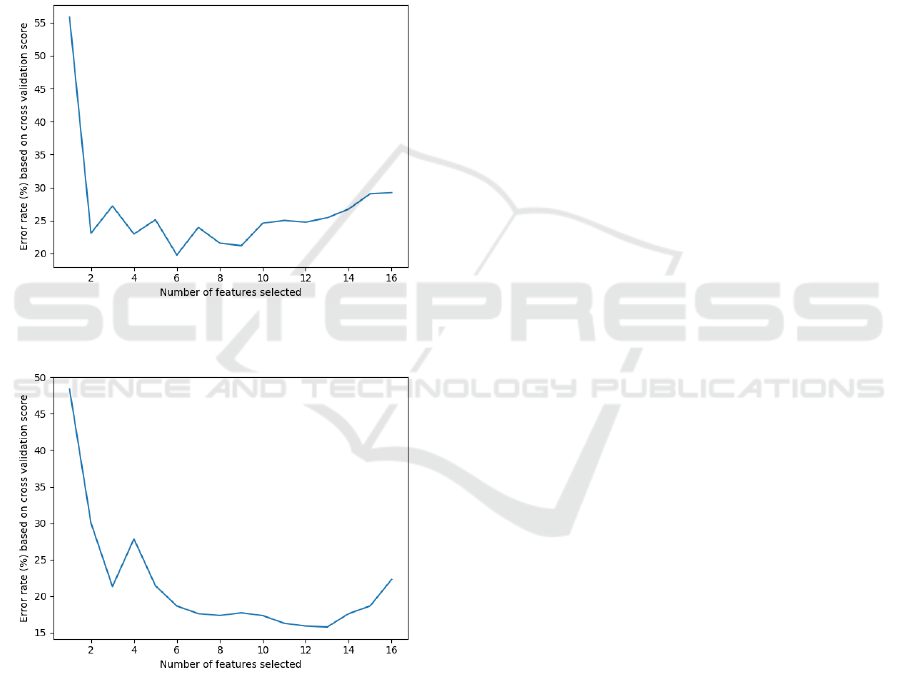
6 features. Consequently, the best number of featu-

res for VOCs classiﬁcation using sensors with sensing

ﬁlms produced by Film Coating is 6.

Figure 7b shows that the best number of features

for VOCs classiﬁcation using sensors with sensing

ﬁlms produced by Spin Coating is also 6. A higher

number of features decreases the error rate. Howe-

ver, the error decreases less than 5 % using 13 featu-

res. Since a lower number of features improves the

computation performance, we decided to use also 6

features for this group of sensors.

Therefore, in the next steps, only the best 6 featu-

res per group were selected.

(a) Features extracted from signals obtained from sen-

sors with sensing ﬁlms produced by Film Coating.

(b) Features extracted from signals obtained from sen-

sors with sensing ﬁlms produced by Spin Coating.

Figure 7: Correlation between cross-validation scores of

RFE vs number of features extracted from signals.

The ranking obtained by RFE indicated that the

6 features with a higher score were: arelv1, mv1,

maxdv1, arelv4, mv4 and maxdv4 for Film Coating;

and arelv3, mv3, maxdv3, mindv3, arelv5, and mv5

for Spin Coating. Therefore, these features were the

only used for training and testing in the classiﬁcation

models performed.

3.2 Classiﬁcation

We studied the best parameter C for Logistic regres-

sion, and the best maximum depth of Decision Tree,

using features extracted from the signals given by sen-

sors where sensing ﬁlms produced by Film Coating

were used, and by sensors where sensing ﬁlms produ-

ced by Spin Coating were used. Then, we assessed the

accuracy of the three classiﬁcation models: Logistic

regression, Decision Tree and Na

ıve Bayes.

3.2.1 Classiﬁcation using Sensors with Sensing

Films Produced by Film Coating

The value of parameter C for Logistic Regression was

optimised - Figure 8a , as well as the best value for

depth in Decision Tree - Figure 8b.

Using sensing ﬁlms produced by Film Coating in

the sensors, the best value of parameter C for Logistic

Regression is 65536 - Figure 8a. And the best depth

for Decision Tree is 15 - Figure 8b. Hence, these va-

lues were selected to be used in the classiﬁers’ mo-

dels.

The estimated errors calculated on the Test set

were 2.75 % for Multinominal Logistic Regression,

3.15 % for Decision Tree, and 3.15 % for Na

ive

Bayes.

We also compared the difference in accuracy bet-

ween the classiﬁers using the McNemar’s test, which

indicates a signiﬁcant difference between two classi-

ﬁers (with 95 % conﬁdence) if the value of the test is

≥ 3.84. The results for Film Coating were the follo-

wing:

• Multinominal Logistic Regression vs Decision

Tree: 0.0

• Multinominal Logistic Regression vs Na

ıve

Bayes: 0.0

• Decision Tree vs Na

ıve Bayes: 0.1

The results above indicate that there is no signiﬁ-

cant difference between the accuracy of the three clas-

siﬁers used.

3.2.2 Classiﬁcation using Sensors with Sensing

Films Produced by Spin Coating

Using sensing ﬁlms produced by Spin Coating in the

sensors, the best value of parameter C for Logistic

Regression is 32768 - Figure 9a. And the best depth

for Decision Tree is 8 - Figure 9b. Hence, these values

were selected to be used in the classiﬁers’ models.

The estimated errors calculated on the Test set

were 2.76 % for Multinominal Logistic Regression,

3.15 % for Decision Tree, and 3.94 % for Na

ive

Bayes.

BIODEVICES 2019 - 12th International Conference on Biomedical Electronics and Devices

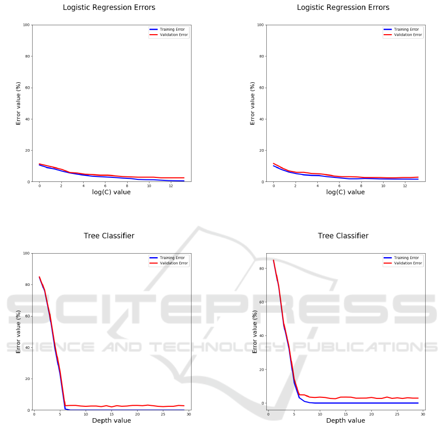
(a) Optimisation of C parameter for Logistic Regression.

(b) Optimisation of depth parameter for Decision Tree.

Figure 8: Optimisation of algorithms’ parameters using sen-

sing ﬁlms produced by Film Coating.

The McNemar’s test was also performed. The re-

sults for Spin Coating were the following:

• Multinominal Logistic Regression vs Decision

Tree: 0.00

• Multinominal Logistic Regression vs Na

ıve

Bayes: 0.36

• Decision Tree vs Na

ıve Bayes: 0.08

The results above indicate that there is no signiﬁ-

cant difference among the accuracy results of Mul-

tinominal Logistic Regression, Decision Tree and

ıve Bayes.

(a) Optimisation of C parameter for Logistic Regression.

(b) Optimisation of depth parameter for Decision Tree.

Figure 9: Optimisation of algorithms’ parameters using sen-

sing ﬁlms produced by Spin Coating.

4 CONCLUSIONS

In this study, the RFE results indicate that the most

effective features for classiﬁcations are: relative am-

plitude, maximum of the signal, and maximum and

minimum of signal’s ﬁrst derivative.

For distinction of 13 different VOCs, the three

simple classiﬁcation methods studied were effective,

with estimated error inferior to 4 % for all of them.

Comparing the results obtained for sensors with

sensing ﬁlms produced by Film Coating vs sensing

Impact of Sensing Film’s Production Method on Classiﬁcation Accuracy by Electronic Nose

ﬁlms produced by Spin Coating, the values did not

vary signiﬁcantly for any of the classiﬁers. Therefore,

we conclude that both spreading method techniques

are very good for sensing ﬁlms production, and none

of them revealed to be better than the others for VOCs

classiﬁcation.

The E-nose system and the machine learning algo-

rithms applied in the present study demonstrated ca-

pability to distinguish the different VOCs in a quick,

simple and accurate way, using both sensing ﬁlm pro-

duction types.

Future studies can be performed in order to ex-

plore the application of the E-nose in many different

sectors, such as food and beverage evaluation, envi-

ronmental safety or medical research. Moreover, ot-

her Machine Learning algorithms can be explored and

optimised.

REFERENCES

Barbri, N. E., Mirhisse, J., Ionescu, R., Bari, N. E., Correig,

X., Bouchikhi, B., and Llobet, E. (2009). An electro-

nic nose system based on a micro-machined gas sen-

sor array to assess the freshness of sardines. Sensors

& Actuators: B. Chemical, 141:538 – 543.

Cho, J. H. and Kurup, P. U. (2011). Decision tree appro-

ach for classiﬁcation and dimensionality reduction of

electronic nose data. Sensors & Actuators: B. Chemi-

cal, 160:542 – 548.

Ghasemi-Varnamkhasti, M., Mohtasebi, S. S., Siadat, M.,

Ahmadi, H., and Razavi, S. H. (2015). Research pa-

per: From simple classiﬁcation methods to machine

learning for the binary discrimination of beers using

electronic nose data. Engineering in Agriculture, En-

vironment and Food, 8:44 – 51.

Gutirrez, J. and Horrillo, M. (2014). Advances in arti-

ﬁcial olfaction: sensors and applications. Talanta,

124:95105.

Hotel, O., Poli, J.-P., Mer-Calfati, C., Scorsone, E., and

Saada, S. (2018). A review of algorithms for saw sen-

sors e-nose based volatile compound identiﬁcation.

Sensors & Actuators: B. Chemical, 255(Part 3):2472

– 2482.

Hussain, A., Semeano, A. T. S., Palma, S. I. C. J., Pina,

A. S., Almeida, J., Medrado, B. F., Padua, A. C. C. S.,

Carvalho, A. L., Dionisio, M., Li, R. W. C., Gam-

boa, H., Ulijn, R. V., Gruber, J., and Roque, A. C. A.

(2017). Liquid crystals: Tunable gas sensing gels

by cooperative assembly (adv. funct. mater. 27/2017).

Advanced Functional Materials, 27(27):n/a.

Ordukaya, E. and Karlik, B. (2017). Quality control of olive

oils using machine learning and electronic nose. Jour-

nal of Food Quality, Vol 2017 (2017).

Padua, A. C., Palma, S., Gruber, J., Gamboa, H., and Ro-

que, A. C. (2018). Design and evolution of an opto-

electronic device for vocs detection. In Proceedings of

the 11th International Joint Conference on Biomedi-

cal Engineering Systems and Technologies - Volume 1:

BIODEVICES,, pages 48–55. INSTICC, SciTePress.

Peris, M. and Escuder-Gilabert, L. (2009). A 21st century

technique for food control: Electronic noses. Analy-

tica Chimica Acta, 638(1):1 – 15.

Phaisangittisagul, E., Nagle, H. T., and Areekul, V. (2010).

Intelligent method for sensor subset selection for ma-

chine olfaction. Sensors & Actuators: B. Chemical,

145:507 – 515.

Polaka, I., Gaenko, E., Barash, O., Haick, H., and Leja, M.

(2017). Constructing interpretable classiﬁers to diag-

nose gastric cancer based on breath tests. Procedia

Computer Science, 104(ICTE 2016, Riga Technical

University, Latvia):279 – 285.

Sankaran, S., Khot, L. R., and Panigrahi, S. (2012). Review:

Biology and applications of olfactory sensing system:

A review. Sensors & Actuators: B. Chemical, 171-

172:1 – 17.

Siavash, E., Alﬁan, W., Ella, M., Ramesh P., A., and Ja-

mes A., C. (2018). Non-invasive diagnosis of diabetes

by volatile organic compounds in urine using faims

and fox4000 electronic nose. Biosensors, Vol 8, Iss 4,

p 121 (2018), (4):121.

Xu, L., He, J., Duan, S., Wu, X., and Wang, Q. (2016).

Comparison of machine learning algorithms for con-

centration detection and prediction of formaldehyde

based on electronic nose. Sensor Review, 36(2):207.

Yan, J., Xiuzhen, G., Shukai, D., Pengfei, J., Lidan, W.,

Chao, P., and Songlin, Z. (2015). Electronic nose fe-

ature extraction methods: A review. Sensors, Vol 15,

Iss 11, Pp 27804-27831 (2015), (11):27804.

Zhang, H., Chang, M., Wang, J., and Ye, S. (2008). Evalua-

tion of peach quality indices using an electronic nose

by mlr, qpst and bp network. Sensors & Actuators: B.

Chemical, 134:332 – 338.

BIODEVICES 2019 - 12th International Conference on Biomedical Electronics and Devices